FAQ on practical implementation of RAID. What are RAID arrays and why are they needed? Why did this happen in general?

27.06.2021 Instructions

The shift in focus from processor-centric to data-centric applications is driving the increased importance of data storage systems. At the same time, the problem of low throughput and fault tolerance characteristic of such systems has always been quite important and always required a solution.

In the modern computer industry, magnetic disks are widely used as a secondary data storage system, because, despite all their shortcomings, they have the best characteristics for the corresponding type of device at an affordable price.

Features of the technology for constructing magnetic disks have led to a significant discrepancy between the increase in performance of processor modules and the magnetic disks themselves. If in 1990 the best among serial ones were 5.25″ drives with an average access time of 12 ms and a latency time of 5 ms (at a spindle speed of about 5,000 rpm 1), then today the palm belongs to 3.5″ drives with an average access time of 5 ms and delay time 1 ms (at spindle speed 10,000 rpm). Here we see an improvement technical characteristics by an amount of about 100%. At the same time, processor performance increased by more than 2,000%. This is largely possible because the processors have the direct benefits of using VLSI (Very Large Scale Integration). Its use not only makes it possible to increase the frequency, but also the number of components that can be integrated into the chip, which makes it possible to introduce architectural advantages that allow parallel computing.

1 - Average data.

The current situation can be characterized as a secondary storage system I/O crisis.

Increasing performance

The impossibility of significantly increasing the technological parameters of magnetic disks entails the need to search for other ways, one of which is parallel processing.

If you arrange a block of data across N disks of some array and organize this placement so that it is possible to read information simultaneously, then this block can be read N times faster (without taking into account the block formation time). Since all data is transferred in parallel, this architectural solution is called parallel-access array(array with parallel access).

Parallel arrays are typically used for applications that require large data transfers.

Some tasks, on the contrary, are characterized by a large number of small requests. Such tasks include, for example, database processing tasks. By distributing database records across array disks, you can distribute the load by positioning the disks independently. This architecture is usually called independent-access array(array with independent access).

Increasing fault tolerance

Unfortunately, as the number of disks in an array increases, the reliability of the entire array decreases. With independent failures and an exponential distribution law of time between failures, the MTTF of the entire array (mean time to failure) is calculated using the formula MTTF array = MMTF hdd /N hdd (MMTF hdd is the mean time to failure of one disk; NHDD is the number disks).

Thus, there is a need to increase the fault tolerance of disk arrays. To increase the fault tolerance of arrays, redundant coding is used. There are two main types of encoding that are used in redundant disk arrays - duplication and parity.

Duplication, or mirroring, is most often used in disk arrays. Simple mirror systems use two copies of data, each copy located on separate disks. This scheme is quite simple and does not require additional hardware costs, but it has one significant drawback - it uses 50% of the disk space to store a copy of information.

The second way to implement redundant disk arrays is to use redundant encoding using parity calculation. Parity is calculated by XORing all the characters in the data word. Using parity in redundant disk arrays reduces overhead to a value calculated by the formula: HP hdd =1/N hdd (HP hdd - overhead; N hdd - number of disks in the array).

History and development of RAID

Despite the fact that storage systems based on magnetic disks have been produced for 40 years, mass production of fault-tolerant systems began only recently. Redundant disk arrays, commonly called RAID (redundant arrays of inexpensive disks), were introduced by researchers (Petterson, Gibson and Katz) at the University of California, Berkeley in 1987. But RAID systems became widespread only when disks that were suitable for use in redundant arrays became available and sufficiently productive. Since the white paper on RAID in 1988, research into redundant disk arrays has exploded in an attempt to provide a wide range of cost-performance-reliability trade-offs.

There was an incident with the abbreviation RAID at one time. The fact is that at the time of writing this article, all disks that were used in PCs were called inexpensive disks, as opposed to expensive disks for mainframes (mainframe computers). But for use in RAID arrays, it was necessary to use rather expensive equipment compared to other PC configurations, so RAID began to be deciphered as redundant array of independent disks 2 - a redundant array of independent disks.

2 - Definition of RAID Advisory Board

RAID 0 was introduced by the industry as the definition of a non-fault-tolerant disk array. Berkeley defined RAID 1 as a mirrored disk array. RAID 2 is reserved for arrays that use Hamming code. RAID levels 3, 4, 5 use parity to protect data from single faults. It was these levels, including level 5, that were presented at Berkeley, and this RAID taxonomy was adopted as a de facto standard.

RAID levels 3,4,5 are quite popular and have good disk space utilization, but they have one significant drawback - they are only resistant to single faults. This is especially true when using a large number of disks, when the likelihood of simultaneous downtime of more than one device increases. In addition, they are characterized by a long recovery, which also imposes some restrictions on their use.

Today, a fairly large number of architectures have been developed that ensure the operation of the array even with the simultaneous failure of any two disks without data loss. Among the whole set, it is worth noting two-dimensional parity and EVENODD, which use parity for encoding, and RAID 6, which uses Reed-Solomon encoding.

In a scheme using dual-space parity, each data block participates in the construction of two independent codewords. Thus, if a second disk in the same codeword fails, a different codeword is used to reconstruct the data.

The minimum redundancy in such an array is achieved with an equal number of columns and rows. And is equal to: 2 x Square (N Disk) (in “square”).

If the two-space array is not organized into a “square,” then when implementing the above scheme, the redundancy will be higher.

The EVENODD architecture has a fault tolerance scheme similar to dual-space parity, but a different placement of information blocks that guarantees minimal redundant capacity utilization. As in dual-space parity, each data block participates in the construction of two independent codewords, but the words are placed in such a way that the redundancy coefficient is constant (unlike the previous scheme) and is equal to: 2 x Square (N Disk).

By using two check characters, parity and non-binary codes, the data word can be designed to provide fault tolerance when a double fault occurs. This design is known as RAID 6. Non-binary code, based on Reed-Solomon encoding, is typically computed using tables or as an iterative process using closed-loop linear registers, a relatively complex operation requiring specialized hardware.

Considering that the use of classic RAID options, which provide sufficient fault tolerance for many applications, often has unacceptably low performance, researchers from time to time implement various moves that help increase the performance of RAID systems.

In 1996, Savage and Wilks proposed AFRAID - A Frequently Redundant Array of Independent Disks. This architecture to some extent sacrifices fault tolerance for performance. In an attempt to compensate for the small-write problem typical of RAID level 5 arrays, it is possible to leave striping without parity calculation for a certain period of time. If the disk designated for parity recording is busy, parity recording is delayed. It has been theoretically proven that a 25% reduction in fault tolerance can increase performance by 97%. AFRAID effectively changes the failure model of single fault tolerant arrays because a codeword that does not have updated parity is susceptible to disk failures.

Instead of sacrificing fault tolerance, you can use traditional performance techniques such as caching. Given that disk traffic is bursty, you can use a writeback cache to store data when the disks are busy. And if the cache memory is made in the form of non-volatile memory, then, in the event of a power failure, the data will be saved. In addition, deferred disk operations make it possible to randomly combine small blocks to perform more efficient disk operations.

There are also many architectures that sacrifice volume to increase performance. Among them are delayed modification on the log disk and various schemes for modifying the logical placement of data into the physical one, which allow you to distribute operations in the array more efficiently.

One of the options is parity logging(parity registration), which involves solving the small-write problem and more effective use disks. Parity logging defers parity changes to RAID 5 by recording them in a FIFO log, which is located partly in the controller's memory and partly on disk. Given that access to a full track is on average 10 times more efficient than access to a sector, parity logging collects large amounts of modified parity data, which are then written together to a disk dedicated to storing parity across the entire track.

Architecture floating data and parity(floating and parity), which allows the physical placement of disk blocks to be reallocated. Free sectors are placed on each cylinder to reduce rotational latency(rotation delays), data and parity are allocated to these free spaces. To ensure operation during a power failure, the parity and data map must be stored in non-volatile memory. If you lose the placement map, all data in the array will be lost.

Virtual stripping- is a floating data and parity architecture using writeback cache. Naturally realizing the positive sides of both.

In addition, there are other ways to improve performance, such as RAID operations. At one time, Seagate built support for RAID operations into its drives with Fiber Chanel and SCSI interfaces. This made it possible to reduce traffic between the central controller and the disks in the array for RAID 5 systems. This was a fundamental innovation in the field of RAID implementations, but the technology did not get a start in life, since some features of Fiber Chanel and SCSI standards weaken the failure model for disk arrays.

For the same RAID 5, the TickerTAIP architecture was introduced. It looks like this - the central control mechanism originator node (initiator node) receives user requests, selects a processing algorithm and then transfers disk work and parity to the worker node (work node). Each worker node processes a subset of the disks in the array. As in the Seagate model, worker nodes transfer data among themselves without the participation of the initiating node. If a worker node fails, the disks it served become unavailable. But if the codeword is constructed in such a way that each of its symbols is processed by a separate worker node, then the fault tolerance scheme repeats RAID 5. To prevent failures of the initiating node, it is duplicated, thus we get an architecture that is resistant to failures of any of its nodes. For all its positive features, this architecture suffers from the “write hole” problem. Which means an error occurs when several users change the codeword at the same time and the node fails.

We should also mention a fairly popular method for quickly restoring RAID - using a free disk (spare). If one of the disks in the array fails, the RAID can be restored using a free disk instead of the failed one. The main feature of this implementation is that the system goes to its previous (fail-safe state without external intervention). When using a distributed sparing architecture, the logical blocks of a spare disk are physically distributed across all disks in the array, eliminating the need to rebuild the array if a disk fails.

In order to avoid the recovery problem typical of classic RAID levels, an architecture called parity declustering(parity distribution). It involves placing fewer logical drives with a large volume to physical disks of a smaller volume, but of a larger quantity. Using this technology, the system's response time to a request during reconstruction is improved by more than half, and reconstruction time is significantly reduced.

Architecture of Basic RAID Levels

Now let's look at the architecture of the basic levels of RAID in more detail. Before considering, let's make some assumptions. To demonstrate the principles of constructing RAID systems, consider a set of N disks (for simplicity, we will assume that N is an even number), each of which consists of M blocks.

We will denote the data - D m,n, where m is the number of data blocks, n is the number of subblocks into which the data block D is divided.

Disks can connect to either one or several data transfer channels. Using more channels increases system throughput.

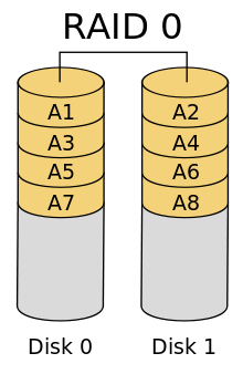
RAID 0. Striped Disk Array without Fault Tolerance

It is a disk array in which data is divided into blocks, and each block is written (or read) to a separate disk. Thus, multiple I/O operations can be performed simultaneously.

Advantages:

highest performance for applications requiring intensive processing of I/O requests and large data volumes;
ease of implementation;
low cost per unit volume.

Flaws:

not a fail-safe solution;
The failure of one drive results in the loss of all data in the array.

RAID 1. Redundant disk array or mirroring

Mirroring is a traditional way to increase the reliability of a small disk array. In the simplest version, two disks are used, on which the same information is recorded, and if one of them fails, a duplicate of it remains, which continues to operate in the same mode.

Advantages:

ease of implementation;
ease of array recovery in case of failure (copying);
sufficiently high performance for applications with high request intensity.

Flaws:

high cost per unit volume - 100% redundancy;
low data transfer speed.

RAID 2. Fault-tolerant disk array using Hamming Code ECC.

The redundant coding used in RAID 2 is called Hamming code. The Hamming code allows you to correct single faults and detect double faults. Today it is actively used in data encoding technology in RAM ECC type. And encoding data on magnetic disks.

IN in this case An example is shown with a fixed number of disks due to the cumbersomeness of the description (a data word consists of 4 bits, respectively, the ECC code is 3).

Advantages:

fast error correction (“on the fly”);
very high data transfer speed for large volumes;
as the number of disks increases, overhead costs decrease;
quite simple implementation.

Flaws:

high cost with a small number of disks;
low request processing speed (not suitable for transaction-oriented systems).

RAID 3. Fault-tolerant array with parallel data transfer and parity (Parallel Transfer Disks with Parity)

Data is broken down into subblocks at the byte level and written simultaneously to all disks in the array except one, which is used for parity. Using RAID 3 solves the problem of high redundancy in RAID 2. Most of the control disks used in RAID level 2 are needed to determine the position of the failed bit. But this is not necessary, since most controllers are able to determine when a disk has failed using special signals, or additional encoding of information written to the disk and used to correct random failures.

Advantages:

very high data transfer speed;
disk failure has little effect on the speed of the array;

Flaws:

difficult implementation;
low performance with high intensity requests for small data.

RAID 4. Fault-tolerant array of independent disks with shared parity disk (Independent Data disks with shared Parity disk)

Data is broken down at the block level. Each block of data is written to a separate disk and can be read separately. Parity for a group of blocks is generated on write and checked on read. RAID Level 4 improves the performance of small data transfers through parallelism, allowing more than one I/O access to be performed simultaneously. The main difference between RAID 3 and 4 is that in the latter, data striping is performed at the sector level, rather than at the bit or byte level.

Advantages:

very high speed of reading large volumes of data;
high performance at high intensity of data reading requests;
low overhead to implement redundancy.

Flaws:

very low performance when writing data;
low speed of reading small data with single requests;
asymmetry of performance regarding reading and writing.

RAID 5. Fault-tolerant array of independent disks with distributed parity blocks

This level is similar to RAID 4, but unlike the previous one, parity is distributed cyclically across all disks in the array. This change improves the performance of writing small amounts of data on multitasking systems. If write operations are planned properly, it is possible to process up to N/2 blocks in parallel, where N is the number of disks in the group.

Advantages:

high data recording speed;
fairly high data reading speed;
high performance at high intensity of data read/write requests;
low overhead to implement redundancy.

Flaws:

Data reading speed is lower than in RAID 4;
low speed of reading/writing small data with single requests;
quite complex implementation;
complex data recovery.

RAID 6. Fault-tolerant array of independent disks with two independent distributed parity schemes (Independent Data disks with two independent distributed parity schemes)

Data is partitioned at the block level, similar to RAID 5, but in addition to the previous architecture, a second scheme is used to improve fault tolerance. This architecture is double fault tolerant. However, when performing a logical write, there are actually six disk accesses, which greatly increases the processing time of one request.

Advantages:

high fault tolerance;
fairly high speed of request processing;
relatively low overhead for implementing redundancy.

Flaws:

very complex implementation;
complex data recovery;
very low data writing speed.

Modern RAID controllers allow you to combine different RAID levels. In this way, it is possible to implement systems that combine the advantages of different levels, as well as systems with a large number of disks. Typically this is a combination of level zero (stripping) and some kind of fault-tolerant level.

RAID 10. Fault-tolerant array with duplication and parallel processing

This architecture is a RAID 0 array whose segments are RAID 1 arrays. It combines very high fault tolerance and performance.

Advantages:

high fault tolerance;
high performance.

Flaws:

very high cost;
limited scaling.

RAID 30. Fault-tolerant array with parallel data transfer and increased performance.

It is a RAID 0 array, the segments of which are RAID 3 arrays. It combines fault tolerance and high performance. Typically used for applications requiring large volumes of serial data transfer.

Advantages:

high fault tolerance;
high performance.

Flaws:

high cost;
limited scaling.

RAID 50: Fault-tolerant array with distributed parity and increased performance

It is a RAID 0 array, the segments of which are RAID 5 arrays. It combines fault tolerance and high performance for applications with high request intensity and high data transfer rates.

Advantages:

high fault tolerance;
high data transfer speed;
high speed of request processing.

Flaws:

high cost;
limited scaling.

RAID 7: Fault-tolerant array optimized for performance. (Optimized Asynchrony for High I/O Rates as well as High Data Transfer Rates). RAID 7® is a registered trademark of Storage Computer Corporation (SCC)

To understand the RAID 7 architecture, let's look at its features:

All data transfer requests are processed asynchronously and independently.
All read/write operations are cached via the high-speed x-bus.
The parity disk can be placed on any channel.
The microprocessor of the array controller uses a real-time operating system focused on processing processes.
The system has good scalability: up to 12 host interfaces and up to 48 disks.
operating system controls communication channels.
Standard SCSI disks, buses, motherboards and memory modules are used.
A high-speed X-bus is used to work with internal cache memory.
The parity generation procedure is integrated into the cache.
Disks attached to the system can be declared as separate.
An SNMP agent can be used to manage and monitor the system.

Advantages:

high data transfer speed and high request processing speed (1.5 - 6 times higher than other standard RAID levels);
high scalability of host interfaces;
the data writing speed increases with the number of disks in the array;
There is no need for additional data transmission to calculate parity.

Flaws:

property of one manufacturer;
very high cost per unit volume;
short warranty period;
cannot be serviced by the user;
you need to use an uninterruptible power supply to prevent data loss from the cache memory.

Let's now look at the standard levels together to compare their characteristics. The comparison is made within the framework of the architectures mentioned in the table.

RAID	Minimum disks	Need in disks	Failure sustainability	Speed data transmission	Intensity processing requests	Practical usage
0	2	N			very high up to N x 1 disk	Graphics, video
1	2	2N*		R > 1 disk W = 1 disk	up to 2 x 1 disk W = 1 disk	small file servers
2	7	2N		~RAID 3	Low	mainframes
3	3	N+1			Low	Graphics, video
4	3	N+1		R W	R=RAID 0 W	file servers
5	3	N+1		R W	R=RAID 0 W	database servers
6	4	N+2	highest	low	R > 1 disk W	used extremely rarely
7	12	N+1		highest	highest	different types applications

Clarifications:

* - the commonly used option is considered;
k - number of subsegments;
R - reading;
W - record.

Some aspects of implementing RAID systems

Let's consider three main options for implementing RAID systems:

software (software-based);
hardware - bus-based;
hardware - autonomous subsystem (subsystem-based).

It is impossible to say unequivocally that any implementation is better than another. Each option for organizing an array satisfies one or another user’s needs, depending on financial capabilities, the number of users and the applications used.

Each of the above implementations is based on the execution of program code. They actually differ in where this code is executed: in the computer’s central processor (software implementation) or in a specialized processor on a RAID controller (hardware implementation).

The main advantage of software implementation is low cost. But at the same time, it has many disadvantages: low performance, load on the central processor with additional work, and increased bus traffic. Usually implemented in software simple levels RAID - 0 and 1, as they do not require significant computation. Taking these features into account, software-based RAID systems are used in entry-level servers.

Hardware RAID implementations accordingly cost more than software ones, since they use additional hardware to perform I/O operations. In doing so, they unload or free up the central processor and system bus and accordingly allow you to increase performance.

Bus-oriented implementations are RAID controllers that use the high-speed bus of the computer in which they are installed (in lately PCI bus is usually used). In turn, bus-oriented implementations can be divided into low-level and high-level. The former usually do not have SCSI chips and use the so-called RAID port on the motherboard with a built-in SCSI controller. In this case, the functions of processing RAID code and I/O operations are distributed between the processor on the RAID controller and the SCSI chips on the motherboard. Thus, the central processor is freed from processing additional code and bus traffic is reduced compared to the software version. The cost of such boards is usually low, especially if they are aimed at RAID 0 or 1 systems (there are also implementations of RAID 3, 5, 10, 30, 50, but they are more expensive), due to which they are gradually displacing software implementations from the entry-level server market. High-level controllers with bus implementation have a slightly different structure than their younger brothers. They take on all functions related to I/O and RAID code execution. In addition, they are not so dependent on the implementation of the motherboard and, as a rule, have more capabilities (for example, the ability to connect a module to store information in the cache in the event of a motherboard failure or power failure). Such controllers are usually more expensive than low-end controllers and are used in mid- and high-end servers. They, as a rule, implement RAID levels 0.1, 3, 5, 10, 30, 50. Considering that bus-oriented implementations are connected directly to the internal PCI bus of the computer, they are the most productive among the systems under consideration (when organizing one- host systems). The maximum performance of such systems can reach 132 MB/s (32bit PCI) or 264 MB/s (64bit PCI) at a bus frequency of 33MHz.

Along with the listed advantages, the bus-oriented architecture has the following disadvantages:

dependence on the operating system and platform;
limited scalability;
limited capabilities for organizing fault-tolerant systems.

All these disadvantages can be avoided by using autonomous subsystems. These systems have completely autonomous external organization and, in principle, are a separate computer that is used to organize information storage systems. In addition, if fiber optic channel technology successfully develops, the performance of autonomous systems will be in no way inferior to bus-oriented systems.

Typically, an external controller is placed in a separate rack and, unlike systems with a bus organization, can have a large number of input/output channels, including host channels, which makes it possible to connect several host computers to the system and organize cluster systems. In systems with a standalone controller, hot standby controllers can be implemented.

One of the disadvantages of autonomous systems is their high cost.

Considering the above, we note that autonomous controllers are usually used to implement high-capacity data storage and cluster systems.

The problem of increasing the reliability of information storage and simultaneously increasing the performance of a data storage system has been on the minds of computer peripheral developers for a long time. Regarding increasing the reliability of storage, everything is clear: information is a commodity, and often very valuable. To protect against data loss, many methods have been invented, the most famous and reliable of which is backup information.

The issue of increasing the performance of the disk subsystem is very complex. The growth in the computing power of modern processors has led to a clear imbalance between the capabilities of hard drives and the needs of processors. At the same time, neither expensive SCSI drives, nor even more so IDE drives, can save you. However, if the capabilities of one disk are not enough, then perhaps partly the solution this problem Will having multiple disks allow it? Of course, the mere presence of two or more hard drives on a computer or server does not change the matter - you need to make these drives work together (in parallel) with each other so that this will improve the performance of the disk subsystem on write/read operations. In addition, is it possible, by using several hard drives, to improve not only performance, but also the reliability of data storage, so that the failure of one of the drives does not lead to loss of information? This is exactly the approach that was proposed back in 1987 by American researchers Patterson, Gibson and Katz from the University of California, Berkeley. In their paper, "A Case for Redundant Arrays of Inexpensive Discs, RAID," they described how multiple low-cost hard drives could be combined into a single logical device, resulting in increased system capacity and performance, and failure of individual disks did not lead to failure of the entire system.

15 years have passed since the article was published, but the technology of building RAID arrays has not lost its relevance today. The only thing that has changed since then is the decoding of the RAID acronym. The fact is that initially RAID arrays were not built on cheap disks at all, so the word Inexpensive (inexpensive) was changed to Independent (independent), which was more true.

Moreover, it is now that RAID technology has become widespread. So, if just a few years ago RAID arrays were used in expensive enterprise-scale servers using SCSI disks, today they have become a kind of de facto standard even for entry-level servers. In addition, the market for IDE RAID controllers is gradually expanding, that is, the task of building RAID arrays on workstations using cheap IDE disks is becoming urgent. Thus, some motherboard manufacturers (Abit, Gigabyte) have already begun to integrate IDE RAID controllers onto the boards themselves.

So, RAID is a redundant array of independent disks (Redundant Arrays of Independent Discs), which is tasked with ensuring fault tolerance and increasing performance. Fault tolerance is achieved through redundancy. That is, part of the disk space capacity is allocated for official purposes, becoming inaccessible to the user.

Increased performance of the disk subsystem is ensured by the simultaneous operation of several disks, and in this sense, the more disks in the array (up to a certain limit), the better.

The joint operation of disks in an array can be organized using either parallel or independent access.

With parallel access, disk space is divided into blocks (strips) for recording data. Similarly, information to be written to disk is divided into the same blocks. When writing, individual blocks are written to different disks (Fig. 1), and several blocks are written to different disks simultaneously, which leads to increased performance in write operations. The necessary information is also read in separate blocks simultaneously from several disks (Fig. 2), which also increases performance in proportion to the number of disks in the array.

It should be noted that the parallel access model is implemented only if the size of the data write request is larger than the size of the block itself. Otherwise, it is simply impossible to implement parallel recording of several blocks. Let's imagine a situation where the size of an individual block is 8 KB, and the size of a request to write data is 64 KB. In this case, the source information is cut into eight blocks of 8 KB each. If you have a four-disk array, you can write four blocks, or 32 KB, at a time. Obviously, in the example considered, the write and read speeds will be four times higher than when using one disk. However, this situation is ideal, since the request size is not always a multiple of the block size and the number of disks in the array.

If the size of the recorded data is less than the block size, then a fundamentally different access model is implemented - independent access. Moreover, this model can also be implemented in the case when the size of the written data is larger than the size of one block. With independent access, all data from a single request is written to a separate disk, that is, the situation is identical to working with one disk. The advantage of the parallel access model is that if several write (read) requests arrive simultaneously, they will all be executed independently, on separate disks (Fig. 3). A similar situation is typical, for example, in servers.

In accordance with different types of access, there are different types of RAID arrays, which are usually characterized by RAID levels. In addition to the type of access, RAID levels differ in the way they accommodate and generate redundant information. Redundant information can either be placed on a specially allocated disk, or shuffled between all disks. There are several more ways to generate this information. The simplest of them is complete duplication (100 percent redundancy), or mirroring. In addition, error correction codes are used, as well as parity calculations.

RAID levels

Currently, there are several standardized RAID levels: from RAID 0 to RAID 5. In addition, combinations of these levels are used, as well as proprietary levels (for example, RAID 6, RAID 7). The most common levels are 0, 1, 3 and 5.

RAID 0

RAID level 0, strictly speaking, is not a redundant array and, accordingly, does not provide reliable data storage. Nevertheless, this level is widely used in cases where it is necessary to ensure high performance of the disk subsystem. This level is especially popular in workstations. When creating a RAID level 0 array, information is divided into blocks, which are written to separate disks (Fig. 4), that is, a system with parallel access is created (if, of course, the block size allows this). By allowing simultaneous I/O from multiple disks, RAID 0 provides the fastest data transfer speeds and maximum disk space efficiency because no storage space is required for checksums. The implementation of this level is very simple. RAID 0 is mainly used in areas where fast transfer of large amounts of data is required.

RAID 1 (Mirrored disk)

RAID Level 1 is an array of disks with 100 percent redundancy. That is, the data is simply completely duplicated (mirrored), due to which very high level reliability (as well as cost). Note that to implement level 1, it is not necessary to first partition the disks and data into blocks. In the simplest case, two disks contain the same information and are one logical disk (Fig. 5). If one disk fails, its functions are performed by another (which is absolutely transparent to the user). In addition, this level doubles the speed of reading information, since this operation can be performed simultaneously from two disks. This information storage scheme is used mainly in cases where the cost of data security is much higher than the cost of implementing a storage system.

RAID 2

RAID Level 2 is a data redundancy scheme that uses Hamming code (see below) for error correction. The written data is not formed on the basis of a block structure, as in RAID 0, but on the basis of words, and the word size is equal to the number of disks for recording data in the array. If, for example, the array has four disks for writing data, then the word size is equal to four disks. Each individual bit of a word is written to a separate disk in the array. For example, if an array has four disks for recording data, then a sequence of four bits, that is, a word, will be written to the disk array in such a way that the first bit will be on the first disk, the second bit on the second, etc.

In addition, an error correction code (ECC) is calculated for each word, which is written to dedicated disks for storing control information (Fig. 6). Their number is equal to the number of bits in the control word, and each bit of the control word is written to a separate disk. The number of bits in the control word and, accordingly, the required number of disks for storing control information is calculated based on the following formula: where K is the bit depth of the data word.

Naturally, when calculating using the specified formula, L is rounded up to the nearest integer. However, in order not to mess with formulas, you can use another mnemonic rule: the bit depth of the control word is determined by the number of bits required for the binary representation of the word size. If, for example, the word size is four (in binary notation 100), then to write this number in binary form, three digits are required, which means the control word size is three. Therefore, if there are four disks to store data, then three more disks will be required to store the control data. Similarly, if you have seven disks for data (in binary notation 111), you will need three disks to store control words. If eight disks are allocated for data (in binary notation 1000), then four disks are needed for control information.

The Hamming code that forms the control word is based on the use of the bitwise “exclusive OR” (XOR) operation (also called “disparity”). Recall that the logical operation XOR gives one if the operands do not match (0 and 1) and zero if they match (0 and 0 or 1 and 1).

The control word itself, obtained using the Hamming algorithm, is the inversion of the result of the bitwise exclusive OR operation of the numbers of those information bits of the word whose values are equal to 1. For illustration, consider the original word 1101. In the first (001), third (011) and fourth (100) The digits of this word are worth one. Therefore, it is necessary to perform a bitwise exclusive OR operation for these bit numbers:

The control word itself (Hamming code) is obtained by bitwise inversion of the resulting result, that is, it is equal to 001.

When reading the data, the Hamming code is again calculated and compared with the source code. To compare two codes, a bitwise “exclusive OR” operation is used. If the comparison result in all bits is zero, then the reading is correct, otherwise its value is the number of the erroneously received bit of the main code. For example, let the source word be 1,100,000. Since the ones are in the sixth (110) and seventh (111) positions, the control word is:

If word 1100100 is recorded during reading, then the control word for it is equal to 101. Comparing the original control word with the received one (bitwise exclusive OR operation), we have:

that is, a reading error in the third position.

Accordingly, knowing exactly which bit is erroneous, it can be easily corrected on the fly.

RAID 2 is one of the few levels that allows you to not only correct single errors on the fly, but also detect double ones. Moreover, it is the most redundant of all levels with correction codes. This data storage scheme is rarely used because it does not cope well with a large number of requests, is complex to organize, and has minor advantages over the RAID 3 level.

RAID 3

RAID Level 3 is a fault-tolerant array with parallel I/O and one additional disk on which control information is written (Figure 7). When recording, the data stream is divided into blocks at the byte level (although possibly at the bit level) and is written simultaneously to all disks of the array, except for the one allocated for storing control information. To calculate the control information (also called a checksum), an exclusive-or (XOR) operation is applied to the data blocks being written. If any disk fails, the data on it can be restored using control data and data remaining on healthy disks.

As an illustration, consider blocks of four bits. Let there be four disks for storing data and one disk for recording checksums. If there is a sequence of bits 1101 0011 1100 1011, divided into blocks of four bits, then to calculate the checksum it is necessary to perform the operation:

Thus, the checksum written to the fifth disk is 1001.

If one of the disks, for example the third, fails, then the block 1100 will be unavailable for reading. However, its value can be easily restored using the checksum and the values of the remaining blocks, using the same “exclusive OR” operation:

Block 3=Block 1Block 2Block 4

Checksum.

In our example we get:

Block 3=1101001110111001= 1100.

RAID Level 3 has much less redundancy than RAID 2. By dividing data into blocks, RAID 3 has high performance. When reading information, the disk is not accessed with checksums (unless there is a failure), which happens every time a write operation occurs. Since each I/O operation accesses virtually all the disks in the array, processing multiple requests simultaneously is not possible. This level is suitable for applications with large files and low access frequency. In addition, the advantages of RAID 3 include a slight decrease in performance in the event of a failure and rapid recovery of information.

RAID 4

RAID Level 4 is a fault-tolerant array of independent disks with one drive for storing checksums (Figure 8). RAID 4 is in many ways similar to RAID 3, but differs from the latter primarily in the significantly larger block size of the data being written (larger than the size of the data being written). This is the main difference between RAID 3 and RAID 4. After writing a group of blocks, a checksum is calculated (in the same way as in the case of RAID 3), which is written to the disk allocated for this purpose. With a larger block size than RAID 3, multiple read operations can be performed simultaneously (independent access design).

RAID 4 improves the performance of small file transfers (by parallelizing the read operation). But since recording must calculate the checksum on the allocated disk, simultaneous operations are impossible here (there is an asymmetry of input and output operations). The level under consideration does not provide speed advantages when transferring large amounts of data. This storage scheme was designed for applications in which data is initially split into small blocks, so there is no need to further split it. RAID 4 is a good solution for file servers where information is primarily read and rarely written. This data storage scheme has a low cost, but its implementation is quite complex, as is data recovery in case of failure.

RAID 5

RAID level 5 is a fault-tolerant array of independent disks with distributed checksum storage (Fig. 9). Data blocks and checksums, which are calculated in the same way as in RAID 3, are written cyclically to all disks of the array, that is, there is no dedicated disk for storing checksum information.

In the case of RAID 5, all disks in the array are the same size, but the total capacity of the disk subsystem available for writing becomes exactly one disk smaller. For example, if five disks are 10 GB in size, then the actual size of the array is 40 GB, since 10 GB is allocated for control information.

RAID 5, like RAID 4, has an independent access architecture, that is, unlike RAID 3, it provides large size logical blocks for storing information. Therefore, as in the case of RAID 4, such an array provides the main benefit when processing several requests simultaneously.

The main difference between RAID 5 and RAID 4 is the way the checksums are placed.

The presence of a separate (physical) disk storing information about checksums, here, as in the three previous levels, leads to the fact that read operations that do not require access to this disk are performed at high speed. However, each write operation changes the information on the control disk, so RAID 2, RAID 3, and RAID 4 do not allow parallel writes. RAID 5 does not have this disadvantage because checksums are written to all disks in the array, allowing multiple reads or writes to be performed simultaneously.

Practical implementation

For practical implementation RAID arrays require two components: the hard drive array itself and the RAID controller. The controller performs the functions of communicating with the server (workstation), generating redundant information when writing and checking when reading, distributing information across disks in accordance with the operating algorithm.

Structurally, controllers can be either external or internal. There are also RAID controllers integrated on the motherboard. In addition, controllers differ in the supported disk interface. Thus, SCSI RAID controllers are intended for use in servers, and IDE RAID controllers are suitable for both entry-level servers and workstations.

A distinctive characteristic of RAID controllers is the number of supported channels for connecting hard drives. Although multiple SCSI drives can be connected to one controller channel, the total throughput The RAID array will be limited by the throughput of one channel, which corresponds to the throughput of the SCSI interface. Thus, the use of multiple channels can significantly improve the performance of the disk subsystem.

When using IDE RAID controllers, the problem of multi-channel becomes even more acute, since two hard drives connected to one channel (more disks are not supported by the interface itself) cannot provide parallel operation - the IDE interface allows you to access only one disk at a certain time. Therefore, IDE RAID controllers must be at least dual-channel. There are also four- and even eight-channel controllers.

Another difference between IDE RAID and SCSI RAID controllers is the number of levels they support. SCSI RAID controllers support all the main levels and, as a rule, several more combined and proprietary levels. The set of levels supported by IDE RAID controllers is much more modest. Usually these are zero and first levels. In addition, there are controllers that support the fifth level and a combination of the first and zero: 0+1. This approach is quite logical, since IDE RAID controllers are designed primarily for workstations, so the main emphasis is on increasing data integrity (level 1) or performance during parallel I/O (level 0). In this case, an independent disk scheme is not needed, since in workstations the flow of write/read requests is much lower than, say, in servers.

The main function of a RAID array is not to increase the capacity of the disk subsystem (as can be seen from its design, the same capacity can be obtained for less money), but to ensure reliable data storage and increase performance. For servers, in addition, there is a requirement for uninterrupted operation, even if one of the drives fails. Uninterrupted operation is ensured by hot swapping, that is, removing a faulty SCSI disk and installing a new one without turning off the power. Because the disk subsystem remains operational (except for level 0) when one drive fails, hot swapping provides recovery that is transparent to users. However, the transfer speed and access speed with one non-working disk are noticeably reduced due to the fact that the controller must recover data from redundant information. True, there is an exception to this rule - RAID systems of levels 2, 3, 4, when a drive with redundant information fails, they begin to work faster! This is natural, since in this case the level “on the fly” changes to zero, which has excellent speed characteristics.

So far, this article has been about hardware solutions. But there is also software offered, for example, by Microsoft for Windows 2000 Server. However, in this case, some initial savings are completely neutralized by the additional load on the central processor, which, in addition to its main work, is forced to distribute data across disks and calculate checksums. Such a solution can be considered acceptable only in the case of a significant excess of computing power and low server load.

Sergey Pakhomov

ComputerPress 3"2002

Today we will find out interesting information about what a RAID array is and what role these arrays play in the life of hard drives, yes, exactly in them.

Hard drives themselves play a fairly important role in a computer, since with the help of them we run the system and store a lot of information on them.

Time passes and anyone hard drive may refuse, it could be any, which we are not talking about today.

I hope that many have heard about the so-called raid arrays, which allow you not only to speed up the operation of hard drives, but also, if something happens, to save important data from disappearing, perhaps forever.

Also, these arrays have serial numbers, which is what makes them different. Each performs different functions. For example, there is RAID 0, 1, 2, 3, 4, 5 etc. Today we will talk about these same arrays, and then I will write an article on how to use some of them.

What is a RAID array?

RAID is a technology that allows you to combine several devices, namely hard drives, in our case there is something like a bunch of them. Thus, we increase the reliability of data storage and read/write speed. Perhaps one of these functions.

So, if you want to either speed up your disk or simply secure your information, it’s up to you. More precisely, it depends on the choice of the desired Raid configuration; these configurations are marked with serial numbers 1, 2, 3...

Raids are very useful feature and I recommend it to everyone. For example, if you use 0 configuration, you will experience an increase in speed hard drive, after all, hard drives are almost the lowest-speed device.

If you ask why, then I think everything is clear. Every year they become more and more powerful, they are equipped with higher frequencies, more cores, and much more. The same with and. But hard drives are only growing in volume so far, but the turnover rate remains the same as 7200. Of course there are also rarer models. The situation has been saved so far by the so-called, which speed up the system several times.

Let's say you came to build RAID 1, in this case you will receive a high guarantee of the protection of your data, since they will be duplicated on another device (disk) and, if one hard drive fails, all the information will remain on the other.

As you can see from the examples, raids are very important and useful, they need to be used.

So, a RAID array is physically a combination of two hard drives connected to system board, maybe three or four. By the way, it should also support the creation of RAID arrays. Connecting hard drives is carried out according to the standard, and the creation of raids takes place at the software level.

When we created the raid programmatically, nothing much changed by eye, you will just work in the BIOS, and everything else will remain as it was, that is, when you look into My Computer, you will see all the same connected drives.

To create an array you don't need much: motherboard with RAID support, two identical hard drives ( this is important). They should be the same not only in volume, but also in cache, interface, etc. It is desirable that the manufacturer be the same. Now turn on the computer and look for the parameter there SATA Configuration and put it on RAID. After restarting the computer, a window should appear in which we will see information about disks and raids. There we have to click CTRL+I to start setting up the raid, that is, adding or removing disks from it. Then its configuration will begin.

How many of these raids are there? There are several of them, namely RAID 1, RAID 2, RAID 3, RAID 4, RAID 5, RAID 6. I will talk in more detail about only two of them.

RAID 0– allows you to create a disk array in order to increase the read/write speed.
RAID 1– allows you to create mirrored disk arrays to protect data.

RAID 0, what is it?

Array RAID 0, which is also called "Stripping" uses from 2 to 4 hard drives, rarely more. Working together, they improve productivity. Thus, the data with such an array is divided into data blocks, and then written to several disks at once.

Performance increases due to the fact that one block of data is written to one disk, to another disk, another block, etc. I think it is clear that 4 disks will increase performance more than two. If we talk about security, it suffers throughout the entire array. If one of the disks fails, then in most cases, all information will be lost forever.

The fact is that in a RAID 0 array, information is located on all disks, that is, the bytes of a file are located on several disks. Therefore, if one disk fails, a certain amount of data will also be lost, and recovery is impossible.

It follows from this that it is necessary to make permanent ones on external media.

RAID 1, what is it?

Array RAID 1, it is also called Mirroring- mirror. If we talk about the disadvantage, then in RAID 1 the volume of one of the hard drives is, as it were, “unavailable” to you, because it is used to duplicate the first drive. In RAID 0 this space is available.

Among the advantages, as you probably already guessed, it follows that the array provides high data reliability, that is, if one disk fails, all the data will remain on the second. Failure of two disks at once is unlikely. Such an array is often used on servers, but this does not prevent it from being used on ordinary computers.

If you choose RAID 1, then know that performance will drop, but if data is important to you, then use a data approach.

RAID 2-6, what is it?

Now I will briefly describe the remaining arrays, so to speak, for general development, and all because they are not as popular as the first two.

RAID 2– needed for arrays that use Hamming code (I wasn’t interested in what kind of code it was). The principle of operation is approximately the same as in RAID 0, that is, information is also divided into blocks and written to disks one by one. The remaining disks are used to store error correction codes, with the help of which, if one of the disks fails, data can be recovered.

True, for of this array It’s better to use 4 disks, which is quite expensive, and as it turned out, when using so many disks, the performance gain is quite controversial.

RAID 3, 4, 5, 6– I will not write about these arrays here, since the necessary information is already on Wikipedia, if you want to know about these arrays, then read it.

Which RAID array to choose?

Let's say you often install various programs, games and copy a lot of music or movies, then you are recommended to use RAID 0. When choosing hard drives, be careful, they must be very reliable so as not to lose information. Be sure to do backups data.

Eat important information, which should be safe and sound? Then RAID 1 comes to the rescue. When choosing hard drives, their characteristics must also be identical.

Conclusion

So we sorted out for some new, and for others old, information on RAID arrays. I hope you find the information useful. Soon I will write about how to create these arrays.

All modern motherboards are equipped with an integrated RAID controller, and top models even have several integrated RAID controllers. The extent to which integrated RAID controllers are in demand by home users is a separate question. In any case, a modern motherboard provides the user with the ability to create a RAID array of several disks. However, not every home user knows how to create a RAID array, what array level to choose, and generally has little idea of the pros and cons of using RAID arrays.
In this article, we will give brief recommendations on creating RAID arrays on home PCs and use a specific example to demonstrate how you can independently test the performance of a RAID array.

History of creation

The term “RAID array” first appeared in 1987, when American researchers Patterson, Gibson and Katz from the University of California Berkeley in their article “A Case for Redundant Arrays of Inexpensive Discs, RAID” described how In this way, you can combine several low-cost hard drives into one logical device so that the resulting capacity and performance of the system are increased, and the failure of individual drives does not lead to failure of the entire system.

More than 20 years have passed since the publication of this article, but the technology of building RAID arrays has not lost its relevance today. The only thing that has changed since then is the decoding of the RAID acronym. The fact is that initially RAID arrays were not built on cheap disks at all, so the word Inexpensive (inexpensive) was changed to Independent (independent), which was more true.

Operating principle

Increased performance of the disk subsystem is ensured by the simultaneous operation of several disks, and in this sense, the more disks in the array (up to a certain limit), the better.

The joint operation of disks in an array can be organized using either parallel or independent access. With parallel access, disk space is divided into blocks (strips) for recording data. Similarly, information to be written to disk is divided into the same blocks. When writing, individual blocks are written to different disks, and multiple blocks are written to different disks simultaneously, which leads to increased performance in write operations. The necessary information is also read in separate blocks simultaneously from several disks, which also increases performance in proportion to the number of disks in the array.

It should be noted that the parallel access model is implemented only if the size of the data write request is larger than the size of the block itself. Otherwise, parallel recording of several blocks is almost impossible. Let's imagine a situation where the size of an individual block is 8 KB, and the size of the request to write data is 64 KB. In this case, the source information is cut into eight blocks of 8 KB each. If you have a four-disk array, you can write four blocks, or 32 KB, at a time. Obviously, in the example considered, the write and read speeds will be four times higher than when using a single disk. This is only true for an ideal situation, but the request size is not always a multiple of the block size and the number of disks in the array.

If the size of the recorded data is less than the block size, then a fundamentally different model is implemented - independent access. Moreover, this model can also be used when the size of the data being written is larger than the size of one block. With independent access, all data from a single request is written to a separate disk, that is, the situation is identical to working with one disk. The advantage of the independent access model is that if several write (read) requests arrive simultaneously, they will all be executed on separate disks independently of each other. This situation is typical, for example, for servers.

In accordance with different types of access, there are different types of RAID arrays, which are usually characterized by RAID levels. In addition to the type of access, RAID levels differ in the way they allocate and generate redundant information. Redundant information can either be placed on a dedicated disk or distributed among all disks. There are many ways to generate this information. The simplest of them is complete duplication (100 percent redundancy), or mirroring. In addition, error correction codes are used, as well as parity calculations.

RAID levels

Currently, there are several RAID levels that can be considered standardized: RAID 0, RAID 1, RAID 2, RAID 3, RAID 4, RAID 5 and RAID 6.

Various combinations of RAID levels are also used, which allows you to combine their advantages. Typically this is a combination of some kind of fault-tolerant level and a zero level used to improve performance (RAID 1+0, RAID 0+1, RAID 50).

Note that all modern RAID controllers support the JBOD (Just a Bench Of Disks) function, which is not intended for creating arrays - it provides the ability to connect individual disks to the RAID controller.

It should be noted that the RAID controllers integrated on motherboards for home PCs do not support all RAID levels. Dual-port RAID controllers only support levels 0 and 1, while RAID controllers with more ports (for example, a 6-port RAID controller integrated in south bridge chipset ICH9R/ICH10R) - also levels 10 and 5.

In addition, if we talk about motherboards based on Intel chipsets, they also implement the Intel Matrix RAID function, which allows you to simultaneously create RAID matrices of several levels on several hard drives, allocating part of the disk space for each of them.