A developer should learn to use the device's graphics processing unit (GPU) effectively so that the application does not slow down or perform unnecessary work.
Configure GPU rendering settings
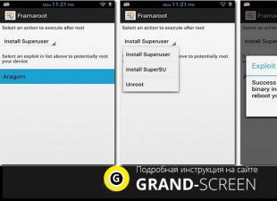
If your application is sluggish, it means that some or all of the screen's refresh frames are taking longer than 16 milliseconds to refresh. To visually see frame updates on the screen, you can enable a special option on the device (Profile GPU Rendering).
You will be able to quickly see how long it takes to render frames. Let me remind you that you need to keep it within 16 milliseconds.
The option is available on devices starting with Android 4.1. Developer mode must be activated on the device. On devices with version 4.2 and higher, the mode is hidden by default. To activate go to Settings | About the phone and click on the line seven times Build number.
After activation, go to Developer Options and find the point Configure GPU rendering settings(Profile GPU rendering) which should be enabled. In the pop-up window, select the option On the screen in the form of columns(On screen as bars). In this case, the graph will be displayed on top of the running application.
You can test not only your application, but also others. Launch any application and start working with it. As you work, you will see an updated graph at the bottom of the screen. The horizontal axis represents elapsed time. The vertical axis shows the time for each frame in milliseconds. When interacting with the application, vertical bars are drawn on the screen, appearing from left to right, showing frame performance over time. Each such column represents one frame for drawing the screen. The higher the column height, the more time it takes to draw. The thin green line is a guide and corresponds to 16 milliseconds per frame. Thus, you need to strive to ensure that the graph does not stray beyond this line when studying your application.
Let's look at a larger version of the graph.
The green line is responsible for 16 milliseconds. To stay within 60 frames per second, each graph bar must be drawn below this line. At some points, the column will be too large and will be much higher than the green line. This means the program is slowing down. Each column has cyan, purple (Lollipop and above), red and orange.
The blue color is responsible for the time used to create and update View.
The purple part represents the time spent transferring the thread's rendering resources.
The red color represents the time to draw.
The orange color shows how long it took the CPU to wait for the GPU to complete its work. This is the source of problems at large values.
There are special techniques to reduce the load on the GPU.
Debug GPU overdraw indicator
Another setting lets you know how often the same portion of the screen is redrawn (i.e., extra work is done). Let's go again Developer Options and find the point Debug GPU overdraw indicator(Debug GPU Overdraw) which should be enabled. In the pop-up window, select the option Show overlay zones(Show overdraw areas). Don't be scared! Some elements on the screen will change color.
Go back to any application and watch it work. The color will indicate problem areas in your application.

If the color in the application has not changed, then everything is fine. There is no layering of one color on top of another.
The blue color indicates that one layer is being drawn on top of the layer below. Fine.
Green color - redrawn twice. You need to think about optimization.
Pink color - redrawn three times. Everything is very bad.
Red color - redrawn many times. Something went wrong.
You can check your application yourself to find problem areas. Create an activity and place a component on it TextView. Give the root element and text label some background in the attribute android:background. You will get the following: first, you painted the bottommost layer of activity with one color. Then a new layer is drawn on top of it from TextView. By the way, actually TextView text is also drawn.
At some points, overlapping colors cannot be avoided. But imagine that you set the background for the list in the same way ListView, which occupies the entire activity area. The system will do double duty, although the user will never see the bottom layer of activity. And if, in addition, you create your own markup for each element of the list with its own background, then you will generally get overkill.
A little advice. Place after method setContentView() calling a method that will remove the screen from being painted with the theme color. This will help remove one extra color overlay:
GetWindow().setBackgroundDrawable(null);
Using GPU Computing with C++ AMP
So far, in discussing parallel programming techniques, we have considered only processor cores. We have acquired some skills in parallelizing programs across multiple processors, synchronizing access to shared resources, and using high-speed synchronization primitives without using locks.
However, there is another way to parallelize programs - graphics processing units (GPUs), with more cores than even high-performance processors. GPU cores are excellent for implementing parallel data processing algorithms, and their large number more than pays for the inconvenience of running programs on them. In this article we will get acquainted with one of the ways to run programs on a GPU, using a set of C++ language extensions called C++AMP.
The C++ AMP extensions are based on the C++ language, which is why this article will demonstrate examples in C++. However, with moderate use of the interaction mechanism in. NET, you can use C++ AMP algorithms in your .NET programs. But we will talk about this at the end of the article.
Introduction to C++ AMP
Essentially, a GPU is the same processor as any other, but with a special set of instructions, a large number of cores and its own memory access protocol. However, there are big differences between modern GPUs and conventional processors, and understanding them is key to creating programs that efficiently use computing power. GPU.
Modern GPUs have a very small instruction set. This implies some limitations: lack of ability to call functions, limited set of supported data types, lack of library functions, and others. Some operations, such as conditional branches, can cost significantly more than similar operations performed on conventional processors. Obviously, moving large amounts of code from the CPU to the GPU under such conditions requires significant effort.
The number of cores in the average GPU is significantly higher than in the average conventional processor. However, some tasks are too small or cannot be broken down into large enough parts to benefit from the GPU.
Synchronization support between GPU cores performing the same task is very poor, and completely absent between GPU cores performing different tasks. This circumstance requires synchronization of the graphics processor with a conventional processor.
The question immediately arises: what tasks are suitable for solving on a GPU? Keep in mind that not every algorithm is suitable for execution on a GPU. For example, GPUs don't have access to I/O devices, so you won't be able to improve the performance of a program that scrapes RSS feeds from the Internet by using a GPU. However, many computational algorithms can be transferred to the GPU and can be massively parallelized. Below are a few examples of such algorithms (this list is by no means complete):
increasing and decreasing sharpness of images, and other transformations;
fast Fourier transform;
matrix transposition and multiplication;
number sorting;
direct hash inversion.
An excellent source for additional examples is the Microsoft Native Concurrency blog, which provides code snippets and explanations for various algorithms implemented in C++ AMP.
C++ AMP is a framework included with Visual Studio 2012 that gives C++ developers an easy way to perform computations on the GPU, requiring only a DirectX 11 driver. Microsoft has released C++ AMP as an open specification that can be implemented by any compiler vendor.
The C++ AMP framework allows you to run code in graphics accelerators, which are computing devices. Using the DirectX 11 driver, the C++ AMP framework dynamically detects all accelerators. C++ AMP also includes a software accelerator emulator and a conventional processor-based emulator, WARP, which serves as a fallback on systems without a GPU or with a GPU but lacks a DirectX 11 driver, and uses multiple cores and SIMD instructions.
Now let's start exploring an algorithm that can easily be parallelized for execution on a GPU. The implementation below takes two vectors of equal length and calculates the pointwise result. It's hard to imagine anything more straightforward:
Void VectorAddExpPointwise(float* first, float* second, float* result, int length) ( for (int i = 0; i< length; ++i) { result[i] = first[i] + exp(second[i]); } }
To parallelize this algorithm on a regular processor, you need to split the iteration range into several subranges and run one thread of execution for each of them. We devoted quite a lot of time in previous articles to exactly this method of parallelizing our first search example prime numbers- we've seen how we can do this by creating threads manually, passing jobs to a thread pool, and using Parallel.For and PLINQ to automatically parallelize. Remember also that when parallelizing similar algorithms on a conventional processor, we took special care not to split the problem into too small tasks.
For the GPU, these warnings are not needed. GPUs have multiple cores that execute threads very quickly, and the cost of context switching is significantly lower than conventional processors. Below is a snippet trying to use the function parallel_for_each from the C++ AMP framework:
#include
Now let's examine each part of the code separately. Let's immediately note that the general form of the main loop has been preserved, but the originally used for loop has been replaced by a call to the parallel_for_each function. In fact, the principle of converting a loop into a function or method call is not new to us - such a technique has previously been demonstrated using the Parallel.For() and Parallel.ForEach() methods from the TPL library.
Next, the input data (parameters first, second and result) are wrapped with instances array_view. The array_view class is used to wrap data passed to the GPU (accelerator). Its template parameter specifies the data type and its dimension. In order to execute instructions on a GPU that access data originally processed on a conventional CPU, someone or something must take care of copying the data to the GPU because most modern graphics cards are separate devices with their own memory. array_view instances solve this problem - they provide data copying on demand and only when it is really needed.
When the GPU completes the task, the data is copied back. By instantiating array_view with a const argument, we ensure that first and second are copied into GPU memory, but not copied back. Likewise, calling discard_data(), we exclude copying result from the memory of a regular processor to the accelerator memory, but this data will be copied in the opposite direction.
The parallel_for_each function takes an extent object that specifies the form of the data to be processed and a function to apply to each element in the extent object. In the example above, we used a lambda function, support for which appeared in the ISO C++2011 (C++11) standard. The restrict (amp) keyword instructs the compiler to check whether the function body can be executed on the GPU and disables most C++ syntax that cannot be compiled into GPU instructions.
Lambda function parameter, index<1>object, represents a one-dimensional index. It must match the extent object being used - if we were to declare the extent object to be two-dimensional (for example, by defining the shape of the source data as a two-dimensional matrix), the index would also need to be two-dimensional. An example of such a situation is given below.
Finally, the method call synchronize() at the end of the VectorAddExpPointwise method, it ensures that the calculation results from array_view avResult, produced by the GPU, are copied back to the result array.
This concludes our first introduction to the world of C++ AMP, and now we are ready for more detailed research, as well as more interesting examples demonstrating the benefits of using parallel computing on a GPU. Vector addition is not a good algorithm and is not the best candidate for demonstrating GPU usage due to the large overhead of copying data. The next subsection will show two more interesting examples.
Matrix multiplication
The first "real" example we'll look at is matrix multiplication. For implementation, we will take a simple cubic matrix multiplication algorithm, and not the Strassen algorithm, which has a execution time close to cubic ~O(n 2.807). Given two matrices, an m x w matrix A and a w x n matrix B, the following program will multiply them and return the result, an m x n matrix C:
Void MatrixMultiply(int* A, int m, int w, int* B, int n, int* C) ( for (int i = 0; i< m; ++i) { for (int j = 0; j < n; ++j) { int sum = 0; for (int k = 0; k < w; ++k) { sum += A * B; } C = sum; } } }
There are several ways to parallelize this implementation, and if you want to parallelize this code to run on a regular processor, the right choice would be to parallelize the outer loop. However, the GPU has a fairly large number of cores, and by parallelizing only the outer loop, we will not be able to create a sufficient number of jobs to load all the cores with work. Therefore, it makes sense to parallelize the two outer loops, leaving the inner loop untouched:
Void MatrixMultiply (int* A, int m, int w, int* B, int n, int* C) ( array_view
This implementation still closely resembles the sequential implementation of matrix multiplication and the vector addition example given above, with the exception of the index, which is now two-dimensional and accessible in the inner loop using the operator. How much faster is this version than the sequential alternative running on a regular processor? Multiplying two matrices (integers) of size 1024 x 1024, the sequential version on a regular CPU takes an average of 7350 milliseconds, while the GPU version - hold on tight - takes 50 milliseconds, 147 times faster!
Particle motion simulation
The examples of solving problems on the GPU presented above have a very simple implementation of the internal loop. It is clear that this will not always be the case. The Native Concurrency blog, linked above, demonstrates an example of modeling gravitational interactions between particles. The simulation involves an infinite number of steps; at each step, new values of the elements of the acceleration vector are calculated for each particle and then their new coordinates are determined. Here, the particle vector is parallelized - with a sufficiently large number of particles (from several thousand and above), you can create a sufficiently large number of tasks to load all the GPU cores with work.
The basis of the algorithm is the implementation of determining the result of interactions between two particles, as shown below, which can easily be transferred to the GPU:
// here float4 are vectors with four elements // representing the particles involved in the operations void bodybody_interaction (float4& acceleration, const float4 p1, const float4 p2) restrict(amp) ( float4 dist = p2 – p1; // no w here used float absDist = dist.x*dist.x + dist.y*dist.y + dist.z*dist.z; float invDist = 1.0f / sqrt(absDist); float invDistCube = invDist*invDist*invDist; = dist*PARTICLE_MASS*invDistCube )
The initial data at each modeling step is an array with the coordinates and velocities of particles, and as a result of calculations, a new array with the coordinates and velocities of particles is created:
Struct particle ( float4 position, velocity; // implementations of constructor, copy constructor and // operator = with restrict(amp) omitted to save space ); void simulation_step(array
With the help of an appropriate graphical interface, modeling can be very interesting. The full example provided by the C++ AMP team can be found on the Native Concurrency blog. On my system with an Intel Core i7 processor and a Geforce GT 740M graphics card, the simulation of 10,000 particles runs at ~2.5 fps (steps per second) using the sequential version running on the regular processor, and 160 fps using the optimized version running on the GPU - a huge increase in performance.
Before we wrap up this section, there is one more important feature of the C++ AMP framework that can further improve the performance of code running on the GPU. GPUs support programmable data cache(often called shared memory). The values stored in this cache are shared by all threads of execution in a single tile. Thanks to memory tiling, programs based on the C++ AMP framework can read data from graphics card memory into the shared memory of the mosaic and then access it from multiple threads of execution without having to re-fetch the data from graphics card memory. Accessing mosaic shared memory is approximately 10 times faster than graphics card memory. In other words, you have reasons to keep reading.
To provide a tiled version of the parallel loop, the parallel_for_each method is passed domain tiled_extent, which divides the multidimensional extent object into multidimensional tiles, and the tiled_index lambda parameter, which specifies the global and local ID of the thread within the tile. For example, a 16x16 matrix can be divided into 2x2 tiles (as shown in the image below) and then passed to the parallel_for_each function:
Extent<2>matrix(16,16); tiled_extent<2,2>tiledMatrix = matrix.tile<2,2>(); parallel_for_each(tiledMatrix, [=](tiled_index<2,2>idx) restrict(amp) ( // ... ));

Each of the four threads of execution belonging to the same mosaic can share the data stored in the block.
When performing operations with matrices, in the GPU core, instead of the standard index<2>, as in the examples above, you can use idx.global. Proper use of local tiled memory and local indexes can provide significant performance gains. To declare tiled memory shared by all threads of execution in a single tile, local variables can be declared with the tile_static specifier.
In practice, the technique of declaring shared memory and initializing its individual blocks in different threads of execution is often used:
Parallel_for_each(tiledMatrix, [=](tiled_index<2,2>idx) restrict(amp) ( // 32 bytes are shared by all threads in the block tile_static int local; // assign a value to the element for this thread of execution local = 42; ));
Obviously, any benefits from using shared memory can only be obtained if access to this memory is synchronized; that is, threads must not access memory until it has been initialized by one of them. Synchronization of threads in a mosaic is performed using objects tile_barrier(reminiscent of the Barrier class from the TPL library) - they will be able to continue execution only after calling the tile_barrier.Wait() method, which will return control only when all threads have called tile_barrier.Wait. For example:
Parallel_for_each(tiledMatrix, (tiled_index<2,2>idx) restrict(amp) ( // 32 bytes are shared by all threads in the block tile_static int local; // assign a value to the element for this thread of execution local = 42; // idx.barrier is an instance of tile_barrier idx.barrier.wait(); // Now this thread can access the "local" array, // using the indexes of other threads of execution ));
Now is the time to translate what you have learned into a concrete example. Let's return to the implementation of matrix multiplication, performed without the use of tiling memory organization, and add the described optimization to it. Let's assume that the matrix size is a multiple of 256 - this will allow us to work with 16 x 16 blocks. The nature of matrices allows for block-by-block multiplication, and we can take advantage of this feature (in fact, dividing matrices into blocks is a typical optimization of the matrix multiplication algorithm, providing more efficient CPU cache usage).
The essence of this technique comes down to the following. To find C i,j (the element in row i and column j in the result matrix), you need to calculate the dot product between A i,* (i-th row of the first matrix) and B *,j (j-th column in the second matrix ). However, this is equivalent to computing the partial dot products of the row and column and then summing the results. We can use this fact to convert the matrix multiplication algorithm into a tiling version:
Void MatrixMultiply(int* A, int m, int w, int* B, int n, int* C) ( array_view The essence of the described optimization is that each thread in the mosaic (256 threads are created for a 16 x 16 block) initializes its element in 16 x 16 local copies of fragments of the original matrices A and B. Each thread in the mosaic requires only one row and one column of these blocks, but all threads together will access each row and each column 16 times. This approach significantly reduces the number of accesses to main memory. To calculate element (i,j) in the result matrix, the algorithm requires the complete i-th row of the first matrix and the j-th column of the second matrix. When the threads are 16x16 tiling represented in the diagram and k=0, the shaded regions in the first and second matrices will be read into shared memory. The execution thread computing element (i,j) in the result matrix will calculate the partial dot product of the first k elements from the i-th row and j-th column of the original matrices. In this example, using a tiled organization provides a huge performance boost. The tiled version of matrix multiplication is much faster than the simple version, taking approximately 17 milliseconds (for the same 1024 x 1024 input matrices), which is 430 times faster than the version running on a conventional processor! Before we end our discussion of the C++ AMP framework, we would like to mention the tools (in Visual Studio) available to developers. Visual Studio 2012 offers a graphics processing unit (GPU) debugger that lets you set breakpoints, examine the call stack, and read and change local variable values (some accelerators support GPU debugging directly; for others, Visual Studio uses a software simulator), and a profiler that lets you evaluate the benefits an application receives from parallelizing operations using a GPU. For more information about debugging capabilities in Visual Studio, see the Walkthrough article. Debugging a C++ AMP Application" on MSDN. So far this article has only shown examples in C++, however, there are several ways to harness the power of the GPU in managed applications. One way is to use interop tools that allow you to offload work with GPU cores to low-level C++ components. This solution is great for those who want to use the C++ AMP framework or have the ability to use pre-built C++ AMP components in managed applications. Another way is to use a library that works directly with the GPU from managed code. There are currently several such libraries. For example, GPU.NET and CUDAfy.NET (both commercial offerings). Below is an example from the GPU.NET GitHub repository demonstrating the implementation of the dot product of two vectors: Public static void MultiplyAddGpu(double a, double b, double c) ( int ThreadId = BlockDimension.X * BlockIndex.X + ThreadIndex.X; int TotalThreads = BlockDimension.X * GridDimension.X; for (int ElementIdx = ThreadId; ElementIdx I am of the opinion that it is much easier and more efficient to learn a language extension (based on C++ AMP) than to try to orchestrate interactions at the library level or make significant changes to the IL language. So, after we looked at the possibilities of parallel programming in .NET and using the GPU, no one doubts that organizing parallel computing is an important way to increase productivity. In many servers and workstations around the world, the invaluable processing power of CPUs and GPUs goes unused because applications simply don't use it. The Task Parallel Library gives us a unique opportunity to include all available CPU cores, although this will require solving some interesting problems of synchronization, excessive task fragmentation, and unequal distribution of work between execution threads. The C++ AMP framework and other multi-purpose GPU parallel computing libraries can be successfully used to parallelize calculations across hundreds of GPU cores. Finally, there is a previously unexplored opportunity to obtain productivity gains from the use of cloud distributed computing technologies, which have recently become one of the main directions in the development of information technology. GPU Computing CUDA technology (Compute Unified Device Architecture) is a software and hardware architecture that allows computing using NVIDIA graphics processors that support GPGPU (random computing on video cards) technology. The CUDA architecture first appeared on the market with the release of the eighth generation NVIDIA chip - G80 and is present in all subsequent series of graphics chips that are used in the GeForce, ION, Quadro and Tesla accelerator families. CUDA SDK allows programmers to implement algorithms executable on NVIDIA GPUs in a special simplified dialect of the C programming language and to include special functions in the text of a C program. CUDA gives the developer the opportunity, at his own discretion, to organize access to the instruction set of the graphics accelerator and manage its memory, and organize complex parallel calculations on it. Story In 2003, Intel and AMD were in a joint race to find the most powerful processor. Over several years, as a result of this race, clock speeds increased significantly, especially after the release of the Intel Pentium 4. After the increase in clock frequencies (between 2001 and 2003, the clock frequency of the Pentium 4 doubled from 1.5 to 3 GHz), and users had to be content with tenths of gigahertz, which were brought to the market by manufacturers (from 2003 to 2005, clock frequencies increased 3 to 3.8 GHz). Architectures optimized for high clock frequencies, such as Prescott, also began to experience difficulties, and not only production ones. Chip makers are faced with challenges in overcoming the laws of physics. Some analysts even predicted that Moore's Law would cease to apply. But that did not happen. The original meaning of the law is often distorted, but it concerns the number of transistors on the surface of the silicon core. For a long time, an increase in the number of transistors in a CPU was accompanied by a corresponding increase in performance - which led to a distortion of the meaning. But then the situation became more complicated. The developers of the CPU architecture approached the law of growth reduction: the number of transistors that needed to be added for the required increase in performance became increasingly large, leading to a dead end. The reason why GPU manufacturers have not encountered this problem is very simple: CPUs are designed to get maximum performance on a stream of instructions that process different data (both integer and floating point numbers), perform random memory access, etc. d. Until now, developers are trying to provide greater parallelism of instructions - that is, execute as many instructions as possible in parallel. For example, with the Pentium, superscalar execution appeared, when under certain conditions it was possible to execute two instructions per clock cycle. Pentium Pro received out-of-order execution of instructions, which made it possible to optimize the operation of computing units. The problem is that there are obvious limitations to executing a sequential stream of instructions in parallel, so blindly increasing the number of computational units does not provide any benefit since they will still be idle most of the time. The operation of the GPU is relatively simple. It consists of taking a group of polygons on one side and generating a group of pixels on the other. Polygons and pixels are independent of each other, so they can be processed in parallel. Thus, in a GPU it is possible to allocate a large part of the crystal into computational units, which, unlike the CPU, will actually be used. GPU differs from CPU not only in this way. Memory access in the GPU is very coupled - if a texel is read, then after a few clock cycles the neighboring texel will be read; When a pixel is recorded, after a few clock cycles the neighboring one will be recorded. By intelligently organizing memory, you can achieve performance close to theoretical throughput. This means that the GPU, unlike the CPU, does not require a huge cache, since its role is to speed up texturing operations. All that is needed is a few kilobytes containing a few texels used in bilinear and trilinear filters. First calculations on GPU The earliest attempts at such applications were limited to the use of certain hardware functions, such as rasterization and Z-buffering. But in the current century, with the advent of shaders, matrix calculations began to be accelerated. In 2003, at SIGGRAPH, a separate section was allocated for GPU computing, and it was called GPGPU (General-Purpose computation on GPU). The best known is BrookGPU, a compiler for the Brook streaming programming language, designed to perform non-graphical computations on the GPU. Before its appearance, developers using the capabilities of video chips for calculations chose one of two common APIs: Direct3D or OpenGL. This seriously limited the use of GPUs, because 3D graphics use shaders and textures that parallel programming specialists are not required to know about; they use threads and cores. Brook was able to help make their task easier. These streaming extensions to the C language, developed at Stanford University, hid the 3D API from programmers, and presented the video chip as a parallel coprocessor. The compiler processed the .br file with C++ code and extensions, producing code linked to a DirectX, OpenGL, or x86-enabled library. The appearance of Brook aroused interest among NVIDIA and ATI and subsequently opened up a whole new sector of it - parallel computers based on video chips. Subsequently, some researchers from the Brook project moved to the NVIDIA development team to introduce a hardware-software parallel computing strategy, opening up new market share. And the main advantage of this NVIDIA initiative is that developers know all the capabilities of their GPUs down to the last detail, and there is no need to use the graphics API, and you can work with the hardware directly using the driver. The result of this team's efforts was NVIDIA CUDA. Areas of application of parallel calculations on GPU When transferring calculations to the GPU, many tasks achieve acceleration of 5-30 times compared to fast general-purpose processors. The largest numbers (on the order of 100x speedup and even more!) are achieved with code that is not very well suited for calculations using SSE blocks, but is quite convenient for GPUs. These are just some examples of speedups for synthetic code on the GPU versus SSE-vectorized code on the CPU (according to NVIDIA): Fluorescence microscopy: 12x. Molecular dynamics (non-bonded force calc): 8-16x; Electrostatics (direct and multilevel Coulomb summation): 40-120x and 7x. A table that NVIDIA displays in all presentations shows the speed of GPUs relative to CPUs. List of the main applications in which GPU computing is used: analysis and processing of images and signals, physics simulation, computational mathematics, computational biology, financial calculations, databases, dynamics of gases and liquids, cryptography, adaptive radiation therapy, astronomy, audio processing, bioinformatics , biological simulations, computer vision, data mining, digital cinema and television, electromagnetic simulations, geographic information systems, military applications, mine planning, molecular dynamics, magnetic resonance imaging (MRI), neural networks, oceanographic research, particle physics, protein folding simulation, quantum chemistry, ray tracing, visualization, radar, reservoir simulation, artificial intelligence, satellite data analysis, seismic exploration, surgery, ultrasound, video conferencing. Advantages and Limitations of CUDA From a programmer's perspective, a graphics pipeline is a collection of processing stages. The geometry block generates the triangles, and the rasterization block generates the pixels displayed on the monitor. The traditional GPGPU programming model looks like this: To transfer calculations to the GPU within this model, a special approach is needed. Even element-wise addition of two vectors will require drawing the figure on the screen or to an off-screen buffer. The figure is rasterized, the color of each pixel is calculated using a given program (pixel shader). The program reads the input data from the textures for each pixel, adds them and writes them to the output buffer. And all these numerous operations are needed for something that is written in a single operator in a regular programming language! Therefore, the use of GPGPU for general purpose computing has the limitation of being too difficult to train developers. And there are enough other restrictions, because a pixel shader is just a formula for the dependence of the final color of a pixel on its coordinate, and the language of pixel shaders is a language for writing these formulas with a C-like syntax. Early GPGPU methods are a neat trick that allows you to use the power of the GPU, but without any of the convenience. The data there is represented by images (textures), and the algorithm is represented by the rasterization process. Of particular note is the very specific model of memory and execution. The software and hardware architecture for GPU computing from NVIDIA differs from previous GPGPU models in that it allows you to write programs for the GPU in real C language with standard syntax, pointers and the need for a minimum of extensions to access the computing resources of video chips. CUDA is independent of graphics APIs, and has some features designed specifically for general purpose computing. Advantages of CUDA over the traditional approach to GPGPU computing CUDA provides access to 16 KB of thread-shared memory per multiprocessor, which can be used to organize a cache with higher bandwidth than texture fetches; More efficient data transfer between system and video memory; No need for graphics APIs with redundancy and overhead; Linear memory addressing, gather and scatter, ability to write to arbitrary addresses; Hardware support for integer and bit operations. Main limitations of CUDA: Lack of recursion support for executable functions; Minimum block width is 32 threads; Closed CUDA architecture owned by NVIDIA. The weaknesses of programming with previous GPGPU methods are that these methods do not use vertex shader execution units in previous non-unified architectures, data is stored in textures and output to an off-screen buffer, and multi-pass algorithms use pixel shader units. GPGPU limitations can include: insufficient use of hardware capabilities, memory bandwidth limitations, lack of scatter operation (gather only), mandatory use of the graphics API. The main advantages of CUDA over previous GPGPU methods stem from the fact that the architecture is designed to make efficient use of non-graphics computing on the GPU and uses the C programming language without requiring algorithms to be ported to a graphics pipeline concept-friendly form. CUDA offers a new path to GPU computing that does not use graphics APIs, offering random memory access (scatter or gather). This architecture does not have the disadvantages of GPGPU and uses all execution units, and also expands capabilities due to integer mathematics and bit shift operations. CUDA opens up some hardware capabilities not available from graphics APIs, such as shared memory. This is a small memory (16 kilobytes per multiprocessor) that thread blocks have access to. It allows you to cache the most frequently accessed data and can provide faster speeds than using texture fetches for this task. Which, in turn, reduces the throughput sensitivity of parallel algorithms in many applications. For example, it is useful for linear algebra, fast Fourier transform, and image processing filters. Memory access is also more convenient in CUDA. The graphics API code outputs data as 32 single-precision floating-point values (RGBA values simultaneously into eight render targets) into predefined areas, and CUDA supports scatter writing - an unlimited number of records at any address. Such advantages make it possible to execute some algorithms on the GPU that cannot be efficiently implemented using GPGPU methods based on graphics APIs. Also, graphics APIs necessarily store data in textures, which requires preliminary packaging of large arrays into textures, which complicates the algorithm and forces the use of special addressing. And CUDA allows you to read data at any address. Another advantage of CUDA is the optimized data exchange between the CPU and GPU. And for developers who want low-level access (for example, when writing another programming language), CUDA offers low-level assembly language programming capabilities. Disadvantages of CUDA One of the few disadvantages of CUDA is its poor portability. This architecture only works on video chips from this company, and not on all of them, but starting with the GeForce 8 and 9 series and the corresponding Quadro, ION and Tesla. NVIDIA cites a figure of 90 million CUDA-compatible video chips. CUDA Alternatives A framework for writing computer programs related to parallel computing on various graphics and central processors. The OpenCL framework includes a programming language that is based on the C99 standard and an application programming interface (API). OpenCL provides instruction-level and data-level parallelism and is an implementation of the GPGPU technique. OpenCL is a completely open standard and is royalty-free for use. The goal of OpenCL is to complement OpenGL and OpenAL, which are open industry standards for 3D computer graphics and audio, by taking advantage of the power of the GPU. OpenCL is developed and maintained by the non-profit consortium Khronos Group, which includes many large companies, including Apple, AMD, Intel, nVidia, Sun Microsystems, Sony Computer Entertainment and others. CAL/IL(Compute Abstraction Layer/Intermediate Language) ATI Stream Technology is a set of hardware and software technologies that enable AMD GPUs to be used in conjunction with a CPU to accelerate many applications (not just graphics). Applications for ATI Stream include computationally intensive applications such as financial analysis or seismic data processing. The use of a stream processor made it possible to increase the speed of some financial calculations by 55 times compared to solving the same problem using only the central processor. NVIDIA does not consider ATI Stream technology a very strong competitor. CUDA and Stream are two different technologies that are at different levels of development. Programming for ATI products is much more complex - their language is more like assembly language. CUDA C, in turn, is a much more high-level language. Writing on it is more convenient and easier. This is very important for large development companies. If we talk about performance, we can see that its peak value in ATI products is higher than in NVIDIA solutions. But again it all comes down to how to get this power. DirectX11 (DirectCompute) An application programming interface that is part of DirectX, a set of APIs from Microsoft that is designed to run on IBM PC-compatible computers running Microsoft Windows operating systems. DirectCompute is designed to perform general-purpose computing on GPUs, an implementation of the GPGPU concept. DirectCompute was originally published as part of DirectX 11, but later became available for DirectX 10 and DirectX 10.1. NVDIA CUDA in the Russian scientific community. As of December 2009, the CUDA software model is taught in 269 universities around the world. In Russia, training courses on CUDA are given at Moscow, St. Petersburg, Kazan, Novosibirsk and Perm State Universities, the International University of the Nature of Society and Man "Dubna", the Joint Institute for Nuclear Research, the Moscow Institute of Electronic Technology, Ivanovo State Energy University, BSTU. V. G. Shukhov, MSTU im. Bauman, Russian Chemical Technical University named after. Mendeleev, Russian Scientific Center "Kurchatov Institute", Interregional Supercomputer Center of the Russian Academy of Sciences, Taganrog Technological Institute (TTI SFU). I once had a chance to talk at the computer market with the technical director of one of the many companies selling laptops. This “specialist” tried to explain, foaming at the mouth, exactly what laptop configuration I needed. The main message of his monologue was that the time of central processing units (CPUs) is over, and now all applications actively use calculations on the graphics processor (GPU), and therefore the performance of a laptop depends entirely on the GPU, and you don’t have to pay any attention to the CPU attention. Realizing that arguing and trying to reason with this technical director was absolutely pointless, I did not waste time and bought the laptop I needed in another pavilion. However, the very fact of such blatant incompetence of the seller struck me. It would be understandable if he was trying to deceive me as a buyer. Not at all. He sincerely believed in what he said. Yes, apparently, marketers at NVIDIA and AMD eat their bread for a reason, and they managed to instill in some users the idea of the dominant role of the graphics processor in a modern computer. The fact that graphics processing unit (GPU) computing is becoming increasingly popular today is beyond doubt. However, this does not at all diminish the role of the central processor. Moreover, if we talk about the vast majority of user applications, then today their performance entirely depends on the performance of the CPU. That is, the vast majority of user applications do not use GPU computing. In general, GPU computing is mainly performed on specialized HPC systems for scientific computing. But user applications that use GPU computing can be counted on one hand. It should be noted right away that the term “GPU computing” in this case is not entirely correct and can be misleading. The fact is that if an application uses GPU computing, this does not mean that the central processor is idle. GPU computing does not involve transferring the load from the central processor to the graphics processor. As a rule, the central processor remains busy, and the use of a graphics processor, along with the central processor, can improve performance, that is, reduce the time it takes to complete a task. Moreover, the GPU itself here acts as a kind of coprocessor for the CPU, but in no case replaces it completely. To understand why GPU computing is not a panacea and why it is incorrect to say that its computing capabilities exceed those of the CPU, it is necessary to understand the difference between a central processor and a graphics processor. CPU cores are designed to execute a single stream of sequential instructions at maximum performance, while GPU cores are designed to quickly execute a very large number of parallel instruction streams. This is the fundamental difference between GPUs and central processors. The CPU is a general-purpose or general-purpose processor optimized for high performance from a single instruction stream that handles both integer and floating-point numbers. In this case, access to memory with data and instructions occurs predominantly randomly. To improve CPU performance, they are designed to execute as many instructions as possible in parallel. For example, for this purpose, the processor cores use an out-of-order instruction execution unit, which makes it possible to reorder instructions out of the order of their arrival, which makes it possible to increase the level of parallelism in the implementation of instructions at the level of one thread. However, this still does not allow parallel execution of a large number of instructions, and the overhead of parallelizing instructions within the processor core turns out to be very significant. This is why general-purpose processors do not have a very large number of execution units. The graphics processor is designed fundamentally differently. It was originally designed to run a huge number of parallel command streams. Moreover, these command streams are parallelized from the start, and there are simply no overhead costs for parallelizing instructions in the GPU. The GPU is designed to render images. To put it simply, it takes a group of polygons as input, carries out all the necessary operations, and produces pixels as output. Processing of polygons and pixels is independent; they can be processed in parallel, separately from each other. Therefore, due to the inherently parallel organization of work, the GPU uses a large number of execution units, which are easy to load, in contrast to the sequential stream of instructions for the CPU. Graphics and central processors also differ in the principles of memory access. In a GPU, access to memory is easily predictable: if a texture texel is read from memory, then after some time the deadline for neighboring texels will come. When recording, the same thing happens: if a pixel is written to the framebuffer, then after a few clock cycles the pixel located next to it will be written. Therefore, the GPU, unlike the CPU, simply does not need a large cache memory, and textures require only a few kilobytes. The principle of working with memory is also different for GPUs and CPUs. So, all modern GPUs have several memory controllers, and the graphics memory itself is faster, so GPUs have much more O greater memory bandwidth compared to universal processors, which is also very important for parallel calculations operating with huge data streams. In universal processors O Most of the chip area is occupied by various command and data buffers, decoding units, hardware branch prediction units, instruction reordering units and cache memory of the first, second and third levels. All these hardware units are needed to speed up the execution of a few command threads by parallelizing them at the processor core level. The execution units themselves take up relatively little space in a universal processor. In a graphics processor, on the contrary, the main area is occupied by numerous execution units, which allows it to simultaneously process several thousand command threads. We can say that, unlike modern CPUs, GPUs are designed for parallel calculations with a large number of arithmetic operations. It is possible to use the computing power of GPUs for non-graphical tasks, but only if the problem being solved allows for the possibility of parallelizing algorithms across hundreds of execution units available in the GPU. In particular, GPU calculations show excellent results when the same sequence of mathematical operations is applied to a large volume of data. In this case, the best results are achieved if the ratio of the number of arithmetic instructions to the number of memory accesses is sufficiently large. This operation places less demands on execution control and does not require the use of large cache memory. There are many examples of scientific calculations where the advantage of the GPU over the CPU in terms of computational efficiency is undeniable. Thus, many scientific applications in molecular modeling, gas dynamics, fluid dynamics, and others are perfectly suited for calculations on the GPU. So, if the algorithm for solving a problem can be parallelized into thousands of individual threads, then the efficiency of solving such a problem using a GPU can be higher than solving it using only a general-purpose processor. However, you cannot so easily transfer the solution of some problem from the CPU to the GPU, if only simply because the CPU and GPU use different commands. That is, when a program is written for a solution on a CPU, the x86 command set is used (or a command set compatible with a specific processor architecture), but for the GPU, completely different command sets are used, which again take into account its architecture and capabilities. When developing modern 3D games, the DirectX and OpenGL APIs are used, allowing programmers to work with shaders and textures. However, using the DirectX and OpenGL APIs for non-graphical computing on the GPU is not the best option. That is why, when the first attempts to implement non-graphical computing on the GPU (General Purpose GPU, GPGPU) began, the BrookGPU compiler arose. Before its creation, developers had to access video card resources through the OpenGL or Direct3D graphics API, which significantly complicated the programming process, as it required specific knowledge - they had to learn the principles of working with 3D objects (shaders, textures, etc.). This was the reason for the very limited use of GPGPU in software products. BrookGPU has become a kind of “translator”. These streaming extensions to the C language hid the 3D API from programmers, and when using it, the need for 3D programming knowledge practically disappeared. The computing power of video cards has become available to programmers in the form of an additional coprocessor for parallel calculations. The BrookGPU compiler processed the file with C code and extensions, building code linked to a library with DirectX or OpenGL support. Thanks in large part to BrookGPU, NVIDIA and ATI (now AMD) took notice of the emerging technology of general-purpose computing on GPUs and began developing their own implementations that provide direct and more transparent access to the compute units of 3D accelerators. As a result, NVIDIA has developed a hardware and software architecture for parallel computing, CUDA (Compute Unified Device Architecture). The CUDA architecture enables non-graphics computing on NVIDIA GPUs. The release of the public beta version of the CUDA SDK took place in February 2007. The CUDA API is based on a simplified dialect of the C language. The CUDA SDK architecture allows programmers to implement algorithms that run on NVIDIA GPUs and include special functions in the C program text. To successfully translate code into this language, the CUDA SDK includes NVIDIA's own nvcc command line compiler. CUDA is cross-platform software for operating systems such as Linux, Mac OS X and Windows. AMD (ATI) has also developed its own version of GPGPU technology, which was previously called ATI Stream, and now AMD Accelerated Parallel Processing (APP). The AMD APP is based on the open industry standard OpenCL (Open Computing Language). The OpenCL standard provides instruction-level and data-level parallelism and is an implementation of the GPGPU technique. It is a completely open standard and is royalty-free for use. Note that AMD APP and NVIDIA CUDA are incompatible with each other, however, the latest version of NVIDIA CUDA also supports OpenCL. Testing GPGPU in video converters So, we found out that CUDA technology is used to implement GPGPU on NVIDIA GPUs, and the APP API is used on AMD GPUs. As already noted, the use of non-graphical computing on the GPU is advisable only if the problem being solved can be parallelized into many threads. However, most user applications do not meet this criterion. However, there are some exceptions. For example, most modern video converters support the ability to use computing on NVIDIA and AMD GPUs. In order to find out how efficiently GPU computing is used in custom video converters, we selected three popular solutions: Xilisoft Video Converter Ultimate 7.7.2, Wondershare Video Converter Ultimate 6.0.3.2 and Movavi Video Converter 10.2.1. These converters support the ability to use NVIDIA and AMD GPUs, and you can disable this feature in the video converter settings, which allows you to evaluate the effectiveness of using the GPU. For video conversion, we used three different videos. The first video was 3 minutes 35 seconds long and 1.05 GB in size. It was recorded in the mkv data storage format (container) and had the following characteristics: The second video had a duration of 4 minutes 25 seconds and a size of 1.98 GB. It was recorded in the MPG data storage format (container) and had the following characteristics: The third video had a duration of 3 minutes 47 seconds and a size of 197 MB. It was written in the MOV data storage format (container) and had the following characteristics: All three test videos were converted using video converters into the MP4 data storage format (H.264 codec) for viewing on the iPad 2 tablet. The output video file resolution was 1280*um*720. Please note that we did not use exactly the same conversion settings in all three converters. That is why it is incorrect to compare the efficiency of video converters themselves based on conversion time. Thus, in the video converter Xilisoft Video Converter Ultimate 7.7.2, the iPad 2 preset - H.264 HD Video was used for conversion. This preset uses the following encoding settings: Wondershare Video Converter Ultimate 6.0.3.2 used the iPad 2 preset with the following additional settings: Movavi Video Converter 10.2.1 used the iPad preset (1280*um*720, H.264) (*.mp4) with the following additional settings: Conversion of each source video was carried out five times on each of the video converters, using both the GPU and only the CPU. After each conversion, the computer rebooted. As a result, each video was converted ten times in each video converter. To automate this routine work, a special utility with a graphical interface was written, which allows you to fully automate the testing process. The testing stand had the following configuration: The operating system Windows 7 Ultimate (64-bit) was installed at the stand. Initially, we tested the processor and all other system components in normal mode. At the same time, the Intel Core i7-3770K processor operated at a standard frequency of 3.5 GHz with Turbo Boost mode activated (the maximum processor frequency in Turbo Boost mode is 3.9 GHz). We then repeated the testing process, but with the processor overclocked to a fixed frequency of 4.5 GHz (without using Turbo Boost mode). This made it possible to identify the dependence of the conversion speed on the processor frequency (CPU). At the next stage of testing, we returned to the standard processor settings and repeated testing with other video cards: Thus, video conversion was carried out on four video cards of different architectures. The senior NVIDIA GeForce 660Ti video card is based on a graphics processor of the same name, coded GK104 (Kepler architecture), produced using a 28 nm process technology. This GPU contains 3.54 billion transistors and has a die area of 294 mm2. Recall that the GK104 graphics processor includes four graphics processing clusters (Graphics Processing Clusters, GPC). GPC clusters are independent devices within the processor and are capable of operating as separate devices, since they have all the necessary resources: rasterizers, geometry engines and texture modules. Each such cluster has two SMX (Streaming Multiprocessor) multiprocessors, but in the GK104 processor one multiprocessor is blocked in one of the clusters, so there are seven SMX multiprocessors in total. Each SMX streaming multiprocessor contains 192 streaming compute cores (CUDA cores), so the GK104 processor has a total of 1344 CUDA cores. In addition, each SMX multiprocessor contains 16 texture units (TMU), 32 special function units (SFU), 32 load-store units (LSU), a PolyMorph engine and much more. The GeForce GTX 460 is based on a GPU coded GF104 based on the Fermi architecture. This processor is manufactured using a 40nm process technology and contains about 1.95 billion transistors. The GF104 GPU includes two GPC graphics processing clusters. Each of them has four SM streaming multiprocessors, but in the GF104 processor in one of the clusters one multiprocessor is locked, so there are only seven SM multiprocessors. Each SM streaming multiprocessor contains 48 streaming compute cores (CUDA cores), so the GK104 processor has a total of 336 CUDA cores. In addition, each SM multiprocessor contains eight texture units (TMU), eight special function units (SFU), 16 load-store units (LSU), a PolyMorph engine and much more. The GeForce GTX 280 GPU is part of the second generation of NVIDIA's Unified GPU Architecture and is very different in architecture from Fermi and Kepler. The GeForce GTX 280 GPU consists of Texture Processing Clusters (TPCs), which, although similar, are very different from the GPC graphics processing clusters in the Fermi and Kepler architectures. There are a total of ten such clusters in the GeForce GTX 280 processor. Each TPC cluster includes three SM streaming multiprocessors and eight texture sampling and filtering units (TMU). Each multiprocessor consists of eight stream processors (SP). Multiprocessors also contain blocks for sampling and filtering texture data, used in both graphics and some computational tasks. Thus, in one TPC cluster there are 24 stream processors, and in the GeForce GTX 280 GPU there are already 240 of them. Summary characteristics of the video cards on NVIDIA GPUs used in testing are presented in the table. The table below does not include the AMD Radeon HD6850 video card, which is quite natural, since its technical characteristics are difficult to compare with NVIDIA video cards. Therefore, we will consider it separately. The AMD Radeon HD6850 GPU, codenamed Barts, is manufactured using a 40nm process technology and contains 1.7 billion transistors. The AMD Radeon HD6850 processor architecture is a unified architecture with an array of common processors for streaming processing of multiple types of data. The AMD Radeon HD6850 processor consists of 12 SIMD cores, each of which contains 16 superscalar stream processor units and four texture units. Each superscalar stream processor contains five general-purpose stream processors. Thus, in total, the AMD Radeon HD6850 GPU has 12*um*16*um*5=960 universal stream processors. The GPU frequency of the AMD Radeon HD6850 video card is 775 MHz, and the effective GDDR5 memory frequency is 4000 MHz. The memory capacity is 1024 MB. So let's look at the test results. Let's start with the first test, when we use the NVIDIA GeForce GTX 660Ti video card and the standard operating mode of the Intel Core i7-3770K processor. In Fig. 1-3 show the results of converting three test videos using three converters in modes with and without a GPU. As can be seen from the testing results, the effect of using the GPU is obvious. For the video converter Xilisoft Video Converter Ultimate 7.7.2, when using a GPU, the conversion time is reduced by 14, 9 and 19% for the first, second and third video, respectively. For Wondershare Video Converter Ultimate 6.0.32, using a GPU reduces conversion time by 10%, 13%, and 23% for the first, second, and third video, respectively. But the converter that benefits most from the use of a graphics processor is Movavi Video Converter 10.2.1. For the first, second and third video, the reduction in conversion time is 64, 81 and 41%, respectively. It is clear that the benefit from using a GPU depends on both the source video and the video conversion settings, which, in fact, is what our results demonstrate. Now let's see what the conversion time gain will be when overclocking the Intel Core i7-3770K processor to 4.5 GHz. If we assume that in normal mode all processor cores are loaded during conversion and in Turbo Boost mode they operate at a frequency of 3.7 GHz, then increasing the frequency to 4.5 GHz corresponds to a frequency overclock of 22%. In Fig. 4-6 show the results of converting three test videos when overclocking the processor in modes using a graphics processor and without. In this case, the use of a graphics processor allows for a gain in conversion time. For the video converter Xilisoft Video Converter Ultimate 7.7.2, when using a GPU, the conversion time is reduced by 15, 9 and 20% for the first, second and third video, respectively. For Wondershare Video Converter Ultimate 6.0.32, using a GPU can reduce conversion time by 10, 10, and 20% for the first, second, and third video, respectively. For Movavi Video Converter 10.2.1, the use of a graphics processor can reduce conversion time by 59, 81 and 40%, respectively. Naturally, it's interesting to see how CPU overclocking can reduce conversion times with and without a GPU. In Fig. Figures 7-9 show the results of comparing the time for converting videos without using a graphics processor in normal processor operation mode and in overclocked mode. Since in this case the conversion is carried out only by the CPU without calculations on the GPU, it is obvious that increasing the processor clock frequency leads to a reduction in conversion time (increase in conversion speed). It is equally obvious that the reduction in conversion speed should be approximately the same for all test videos. Thus, for the video converter Xilisoft Video Converter Ultimate 7.7.2, when overclocking the processor, the conversion time is reduced by 9, 11 and 9% for the first, second and third video, respectively. For Wondershare Video Converter Ultimate 6.0.32, conversion time is reduced by 9, 9 and 10% for the first, second and third video, respectively. Well, for the video converter Movavi Video Converter 10.2.1, the conversion time is reduced by 13, 12 and 12%, respectively. Thus, when overclocking the processor frequency by 20%, the conversion time is reduced by approximately 10%. Let's compare the time for converting videos using a graphics processor in normal processor mode and in overclocking mode (Fig. 10-12). For the video converter Xilisoft Video Converter Ultimate 7.7.2, when overclocking the processor, the conversion time is reduced by 10, 10 and 9% for the first, second and third video, respectively. For Wondershare Video Converter Ultimate 6.0.32, conversion time is reduced by 9, 6 and 5% for the first, second and third video, respectively. Well, for the video converter Movavi Video Converter 10.2.1, the conversion time is reduced by 0.2, 10 and 10%, respectively. As you can see, for the converters Xilisoft Video Converter Ultimate 7.7.2 and Wondershare Video Converter Ultimate 6.0.32, the reduction in conversion time when overclocking the processor is approximately the same both when using a graphics processor and without using it, which is logical, since these converters do not use very efficiently GPU computing. But for the Movavi Video Converter 10.2.1, which effectively uses GPU computing, overclocking the processor in the GPU computing mode has little effect on reducing the conversion time, which is also understandable, since in this case the main load falls on the graphics processor. Now let's look at the test results with various video cards. It would seem that the more powerful the video card and the more CUDA cores (or universal stream processors for AMD video cards) in the graphics processor, the more effective video conversion should be when using a graphics processor. But in practice it doesn’t work out quite like that. As for video cards based on NVIDIA GPUs, the situation is as follows. When using Xilisoft Video Converter Ultimate 7.7.2 and Wondershare Video Converter Ultimate 6.0.32 converters, the conversion time practically does not depend in any way on the type of video card used. That is, for the NVIDIA GeForce GTX 660Ti, NVIDIA GeForce GTX 460 and NVIDIA GeForce GTX 280 video cards in the GPU computing mode, the conversion time is the same (Fig. 13-15). Rice. 1. Results of converting the first Rice. 14. Results of comparison of conversion time of the second video Rice. 15. Results of comparison of conversion time of the third video This can only be explained by the fact that the GPU calculation algorithm implemented in the Xilisoft Video Converter Ultimate 7.7.2 and Wondershare Video Converter Ultimate 6.0.32 converters is simply ineffective and does not allow active use of all graphics cores. By the way, this is precisely what explains the fact that for these converters the difference in conversion time in modes of using the GPU and without using it is small. In Movavi Video Converter 10.2.1 the situation is slightly different. As we remember, this converter is capable of very efficient use of GPU calculations, and therefore, in GPU mode, the conversion time depends on the type of video card used. But with the AMD Radeon HD 6850 video card everything is as usual. Either the video card driver is “crooked”, or the algorithms implemented in the converters need serious improvement, but when GPU computing is used, the results either do not improve or get worse. More specifically, the situation is as follows. For Xilisoft Video Converter Ultimate 7.7.2, when using a GPU to convert the first test video, the conversion time increases by 43%, and when converting the second video, by 66%. Moreover, Xilisoft Video Converter Ultimate 7.7.2 is also characterized by unstable results. The variation in conversion time can reach 40%! That is why we repeated all tests ten times and calculated the average result. But for Wondershare Video Converter Ultimate 6.0.32 and Movavi Video Converter 10.2.1, when using a GPU to convert all three videos, the conversion time does not change at all! It is likely that Wondershare Video Converter Ultimate 6.0.32 and Movavi Video Converter 10.2.1 either do not use AMD APP technology when converting, or the AMD video driver is simply “crooked”, as a result of which AMD APP technology does not work. Based on the testing, the following important conclusions can be drawn. Modern video converters can actually use GPU computing technology, which allows for increased conversion speed. However, this does not mean that all calculations are entirely transferred to the GPU and the CPU remains unused. As testing shows, when using GPGPU technology, the central processor remains busy, which means that the use of powerful, multi-core central processors in systems used for video conversion remains relevant. The exception to this rule is AMD APP technology on AMD GPUs. For example, when using Xilisoft Video Converter Ultimate 7.7.2 with activated AMD APP technology, the load on the CPU is indeed reduced, but this leads to the fact that the conversion time is not reduced, but, on the contrary, increases. In general, if we talk about converting video with the additional use of a graphics processor, then to solve this problem it is advisable to use video cards with NVIDIA GPUs. As practice shows, only in this case can you achieve an increase in conversion speed. Moreover, you need to remember that the real increase in conversion speed depends on many factors. These are the input and output video formats, and, of course, the video converter itself. The converters Xilisoft Video Converter Ultimate 7.7.2 and Wondershare Video Converter Ultimate 6.0.32 are not suitable for this task, but the converter and Movavi Video Converter 10.2.1 are able to very effectively use the capabilities of the NVIDIA GPU. As for video cards on AMD GPUs, they should not be used for video conversion tasks at all. At best, this will not give any increase in conversion speed, and at worst, you can get a decrease in it. Today, news about the use of GPUs for general computing can be heard on every corner. Words such as CUDA, Stream and OpenCL have become almost the most cited words on the IT Internet in just two years. However, not everyone knows what these words mean and what the technologies behind them mean. And for Linux users, who are accustomed to “being on the fly,” all this seems like a dark forest. Birth of GPGPU We are all used to thinking that the only component of a computer capable of executing any code it is told to do is the central processor. For a long time, almost all mass-produced PCs were equipped with a single processor that handled all conceivable calculations, including the operating system code, all our software and viruses. Later, multi-core processors and multiprocessor systems appeared, in which there were several such components. This allowed machines to perform multiple tasks simultaneously, and the overall (theoretical) system performance increased exactly as much as the number of cores installed in the machine. However, it turned out that it was too difficult and expensive to produce and design multi-core processors. Each core had to house a full-fledged processor of a complex and intricate x86 architecture, with its own (rather large) cache, instruction pipeline, SSE blocks, many blocks that perform optimizations, etc. and so on. Therefore, the process of increasing the number of cores slowed down significantly, and white university coats, for whom two or four cores were clearly not enough, found a way to use other computing power for their scientific calculations, which was abundant on the video card (as a result, the BrookGPU tool even appeared, emulating an additional processor using DirectX and OpenGL function calls). Graphics processors, devoid of many of the disadvantages of the central processor, turned out to be an excellent and very fast calculating machine, and very soon GPU manufacturers themselves began to take a closer look at the developments of scientific minds (and nVidia actually hired most of the researchers to work for them). The result was nVidia CUDA technology, which defines an interface with which it became possible to transfer the calculation of complex algorithms to the shoulders of the GPU without any crutches. Later it was followed by ATi (AMD) with its own version of the technology called Close to Metal (now Stream), and very soon a standard version from Apple appeared, called OpenCL. Is the GPU everything? Despite all the advantages, the GPGPU technique has several problems. The first of these is the very narrow scope of application. GPUs have gone far ahead of the central processor in terms of increasing computing power and the total number of cores (video cards carry a computing unit consisting of more than a hundred cores), but such high density is achieved by maximizing the simplification of the design of the chip itself. In essence, the main task of the GPU comes down to mathematical calculations using simple algorithms that receive not very large amounts of predictable data as input. For this reason, GPU cores have a very simple design, scanty cache sizes and a modest set of instructions, which ultimately results in their low cost of production and the possibility of very dense placement on the chip. GPUs are like a Chinese factory with thousands of workers. They do some simple things quite well (and most importantly, quickly and cheaply), but if you entrust them with assembling an airplane, the result will be, at most, a hang glider. Therefore, the first limitation of GPUs is their focus on fast mathematical calculations, which limits the scope of application of GPUs to assistance in multimedia applications, as well as any programs involved in complex data processing (for example, archivers or encryption systems, as well as software involved in fluorescence microscopy, molecular dynamics, electrostatics and other things of little interest to Linux users). The second problem with GPGPU is that not every algorithm can be adapted for execution on the GPU. Individual GPU cores are quite slow, and their power only becomes apparent when working together. This means that the algorithm will be as effective as the programmer can parallelize it effectively. In most cases, only a good mathematician can handle such work, of which there are very few software developers. And third, GPUs work with memory installed on the video card itself, so each time the GPU is used, there will be two additional copy operations: input data from the RAM of the application itself, and output data from GRAM back to application memory. As you can imagine, this can negate any benefit in application runtime (as is the case with the FlacCL tool, which we'll look at later). But that's not all. Despite the existence of a generally accepted standard in the form of OpenCL, many programmers still prefer to use vendor-specific implementations of the GPGPU technique. CUDA turned out to be especially popular, which, although it provides a more flexible programming interface (by the way, OpenCL in nVidia drivers is implemented on top of CUDA), but tightly ties the application to video cards from one manufacturer. KGPU or Linux kernel accelerated by GPU
Researchers at the University of Utah have developed a KGPU system that allows some Linux kernel functions to be executed on a GPU using the CUDA framework. To perform this task, a modified Linux kernel and a special daemon are used that runs in user space, listens to kernel requests and passes them to the video card driver using the CUDA library. Interestingly, despite the significant overhead that such an architecture creates, the authors of KGPU managed to create an implementation of the AES algorithm, which increases the encryption speed of the eCryptfs file system by 6 times.
What is there now? Due to its youth, and also due to the problems described above, GPGPU has never become a truly widespread technology, but useful software that uses its capabilities exists (albeit in tiny quantities). Crackers of various hashes were among the first to appear, the algorithms of which are very easy to parallelize. Multimedia applications were also born, such as the FlacCL encoder, which allows you to transcode an audio track into the FLAC format. Some pre-existing applications have also acquired GPGPU support, the most notable of which is ImageMagick, which can now offload some of its work to the GPU using OpenCL. There are also projects to transfer data archivers and other information compression systems to CUDA/OpenCL (ATi Unixoids are not liked). We will look at the most interesting of these projects in the following sections of the article, but for now let’s try to figure out what we need to get it all started and working stably. GPUs have long surpassed x86 processors in performance · Secondly, the latest proprietary drivers for the video card must be installed in the system; they will provide support for both GPGPU technologies native to the card and open OpenCL. · And thirdly, since distribution developers have not yet begun to distribute application packages with GPGPU support, we will have to build applications ourselves, and for this we need official SDKs from manufacturers: CUDA Toolkit or ATI Stream SDK. They contain the header files and libraries necessary for building applications. Install CUDA Toolkit Follow the link above and download the CUDA Toolkit for Linux (you can choose from several versions, for the Fedora, RHEL, Ubuntu and SUSE distributions, there are versions for both x86 and x86_64 architectures). In addition, you also need to download driver kits for developers there (Developer Drivers for Linux, they are first on the list). Launch the SDK installer: $ sudo sh cudatoolkit_4.0.17_linux_64_ubuntu10.10.run When the installation is complete, we proceed to installing the drivers. To do this, shut down the X server: # sudo /etc/init.d/gdm stop Open the console $ sudo sh devdriver_4.0_linux_64_270.41.19.run After the installation is complete, start X: In order for applications to be able to work with CUDA/OpenCL, we set the path to the directory with CUDA libraries in the LD_LIBRARY_PATH variable: $ export LD_LIBRARY_PATH=/usr/local/cuda/lib64 Or, if you installed the 32-bit version: $ export LD_LIBRARY_PATH=/usr/local/cuda/lib32 You also need to specify the path to the CUDA header files so that the compiler finds them at the application build stage: $ export C_INCLUDE_PATH=/usr/local/cuda/include That's it, now you can start building CUDA/OpenCL software. Install ATI Stream SDK Stream SDK does not require installation, so you can simply unpack the AMD archive downloaded from the website into any directory (/opt is the best choice) and write the path to it in the same LD_LIBRARY_PATH variable: $ wget http://goo.gl/CNCNo $ sudo tar -xzf ~/AMD-APP-SDK-v2.4-lnx64.tgz -C /opt $ export LD_LIBRARY_PATH=/opt/AMD-APP-SDK-v2.4-lnx64/lib/x86_64/ $ export C_INCLUDE_PATH=/opt/AMD-APP-SDK-v2.4-lnx64/include/ As with the CUDA Toolkit, x86_64 must be replaced with x86 on 32-bit systems. Now go to the root directory and unpack the icd-registration.tgz archive (this is a kind of free license key): $ sudo tar -xzf /opt/AMD-APP-SDK-v2.4-lnx64/icd-registration.tgz - WITH / We check the correct installation/operation of the package using the clinfo tool: $ /opt/AMD-APP-SDK-v2.4-lnx64/bin/x86_64/clinfo ImageMagick and OpenCL OpenCL support has been available in ImageMagick for quite some time, but it is not enabled by default in any distribution. Therefore, we will have to compile IM ourselves from source. There is nothing complicated about this, everything you need is already in the SDK, so the assembly does not require installing any additional libraries from nVidia or AMD. So, download/unpack the archive with the sources: $ wget http://goo.gl/F6VYV $ tar -xjf ImageMagick-6.7.0-0.tar.bz2 $ cd ImageMagick-6.7.0-0 $ sudo apt-get install build-essential We launch the configurator and grab its output for OpenCL support: $ LDFLAGS=-L$LD_LIBRARY_PATH ./confi gure | grep -e cl.h -e OpenCL The correct output from the command should look something like this: checking CL/cl.h usability... yes checking CL/cl.h presence... yes checking for CL/cl.h... yes checking OpenCL/cl.h usability... no checking OpenCL/cl.h presence... no checking for OpenCL/cl.h... no checking for OpenCL library... -lOpenCL The word "yes" must be marked either in the first three lines or in the second (or both options at once). If this is not the case, then most likely the C_INCLUDE_PATH variable was not initialized correctly. If the last line is marked with the word "no", then the problem is in the LD_LIBRARY_PATH variable. If everything is ok, start the build/installation process: $ sudo make install clean Let's check that ImageMagick was actually compiled with OpenCL support: $ /usr/local/bin/convert -version | grep Features Features: OpenMP OpenCL Now let's measure the resulting speed gain. The ImageMagick developers recommend using the convolve filter for this: $ time /usr/bin/convert image.jpg -convolve "-1, -1, -1, -1, 9, -1, -1, -1, -1" image2.jpg $ time /usr/local/bin/convert image.jpg -convolve "-1, -1, -1, -1, 9, -1, -1, -1, -1" image2.jpg Some other operations, such as resizing, should now also work much faster, but you shouldn't expect ImageMagick to start processing graphics at breakneck speed. So far, a very small part of the package has been optimized using OpenCL. FlacCL (Flacuda) FlacCL is an encoder of audio files in the FLAC format, using the capabilities of OpenCL in its work. It is included in the CUETools package for Windows, but thanks to mono it can also be used on Linux. To obtain an archive with an encoder, run the following command: $ mkdir flaccl && cd flaccl $ wget www.cuetools.net/install/flaccl03.rar $ sudo apt-get install unrar mono $ unrar x fl accl03.rar So that the program can find the OpenCL library, we make a symbolic link: $ ln -s $LD_LIBRARY_PATH/libOpenCL.so libopencl.so Now let's run the encoder: $ mono CUETools.FLACCL.cmd.exe music.wav If the error message "Error: Requested compile size is bigger than the required workgroup size of 32" is displayed on the screen, then the video card in our system is too weak, and the number of involved cores should be reduced to the specified number using the '-- flag group-size XX', where XX is the required number of cores. I’ll say right away that due to the long initialization time of OpenCL, noticeable gains can only be obtained on sufficiently long tracks. FlacCL processes short audio files at almost the same speed as its traditional version. oclHashcat or quick brute force As I already said, the developers of various crackers and brute-force password systems were among the first to add GPGPU support to their products. For them, the new technology became a real holy grail, which made it possible to easily transfer naturally easily parallelized code to the shoulders of fast GPU processors. Therefore, it is not surprising that there are now dozens of different implementations of such programs. But in this article I will talk about only one of them - oclHashcat. oclHashcat is a hacker that can guess passwords using their hash at extremely high speed, using the power of the GPU using OpenCL. If you believe the measurements published on the project website, the speed of selecting MD5 passwords on the nVidia GTX580 is up to 15,800 million combinations per second, thanks to which oclHashcat is able to find an average complexity eight-character password in just 9 minutes. The program supports OpenCL and CUDA, MD5, md5($pass.$salt), md5(md5($pass)), vBulletin algorithms< v3.8.5, SHA1, sha1($pass.$salt), хэши MySQL, MD4, NTLM, Domain Cached Credentials, SHA256, поддерживает распределенный подбор паролей с задействованием мощности нескольких машин. $7z x oclHashcat-0.25.7z $cd oclHashcat-0.25 And run the program (we’ll use a sample list of hashes and a sample dictionary): $ ./oclHashcat64.bin example.hash ?l?l?l?l example.dict oclHashcat will open the text of the user agreement, which you must agree to by typing "YES". After this, the search process will begin, the progress of which can be found by pressing To resume - $ ./oclHashcat64.bin hash.txt ?l?l?l?l ?l?l?l?l And various modifications of the dictionary and the direct search method, as well as their combinations (you can read about this in the file docs/examples.txt). In my case, the speed of searching through the entire dictionary was 11 minutes, while direct searching (from aaaaaaaa to zzzzzzzz) lasted about 40 minutes. The average speed of the GPU (RV710 chip) was 88.3 million/s. conclusions Despite many different limitations and the complexity of software development, GPGPU is the future of high-performance desktop computers. But the most important thing is that you can use the capabilities of this technology right now, and this applies not only to Windows machines, but also to Linux.
GPU Computing Alternatives in .NET


Differences in GPU and CPU architectures
NVIDIA CUDA and AMD APP
Test stand configuration
Test results

test video in normal mode
processor operationprocessor on video cards in GPU mode


on various video cards in GPU modeconclusions
. To pause the process, click